A year ago, the same hardware ran everything
Small clusters or individual GPUs support both training and inference during early ML team development. The workloads are small enough that the distinction barely matters. A training run finishes in hours, and inference serves a handful of internal users at volumes that wouldn’t stress a laptop.
Then the model grows, the user base scales, and suddenly the team discovers that the hardware configuration optimized for training throughput is producing unacceptable inference latency — or that the low-latency inference setup can’t sustain the compute throughput needed for a reasonable training cycle. It’s not that the hardware broke. It’s that training and inference are fundamentally different workloads, and the system design that serves one well may serve the other poorly.
Different workloads, different bottlenecks
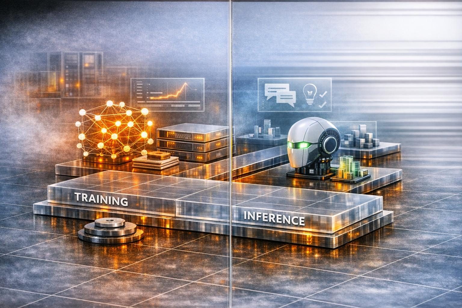
Training versus inference: the two workloads diverge across virtually every hardware and system design axis.
Compute vs. memory pressure. Training is dominated by large matrix multiplications in the forward and backward pass — dense, regular, highly parallelizable operations that saturate compute units efficiently. Modern training runs on large batch sizes, which amortize overhead and keep tensor cores busy. Inference, especially autoregressive decoding in LLMs, is dominated by memory reads. Each token generation reads model weights and KV cache from HBM. The compute-to-memory ratio is radically different: training is compute-bound; much of inference is memory-bandwidth-bound.
Batch dynamics. Training typically processes fixed, large batches. The batch size is tuned for throughput and convergence, and it remains stable through the run. Inference serves variable-length requests that arrive at unpredictable intervals. Batch formation in inference — dynamic batching, continuous batching, iteration-level scheduling — is a system design problem with no training analog.
Latency sensitivity. In training, wall-clock time matters but per-sample latency does not. Nobody cares if a single gradient step takes 200ms instead of 180ms, as long as epoch throughput meets the schedule. In inference, per-request latency directly affects user experience. A P99 latency of 500ms might be acceptable; 2 seconds might not. The optimization target shifts from aggregate throughput to latency distribution — a fundamentally different objective.
Batch size is where this divergence becomes most visible. In training, a larger batch is almost always better: it amortizes overhead, keeps tensor cores saturated, and improves aggregate throughput with no latency penalty to worry about. In inference, batch size cuts both ways — larger batches raise throughput but inflate per-request latency, because a request waits for the batch to form and for slower peers in the same batch to finish. The same lever that is purely beneficial in training becomes a throughput-versus-latency trade-off in inference, which is why continuous batching and iteration-level scheduling exist at all.
Precision requirements. Training often uses mixed precision (FP32 for master weights, BF16 or FP16 for forward/backward computation) to balance numerical stability with throughput. Inference can frequently operate at lower precision — INT8, FP8, even INT4 with careful quantization — because the model weights are frozen and the numerical tolerance for individual predictions is typically higher than for gradient accumulation.
How training and inference differ as workloads
| Dimension | Training | Inference |
|---|---|---|
| Compute profile | Dense matrix ops (forward + backward); compute-bound | Weight and KV cache reads; often memory-bandwidth-bound |
| Batch behavior | Fixed large batches, tuned for throughput and convergence | Variable requests, dynamic batching, continuous batching |
| Latency sensitivity | Per-sample latency irrelevant; epoch throughput matters | Per-request latency directly affects user experience |
| Precision | Mixed precision (FP32 master weights, BF16/FP16 compute) | Lower precision viable (INT8, FP8, INT4 with calibration) |
| Scaling priority | GPU-to-GPU interconnect bandwidth for gradient sync | Memory bandwidth, host-device communication, scheduling efficiency |
| System design | NVLink/InfiniBand, large HBM, sustained power delivery | High memory bandwidth, low-latency host I/O, power efficiency |
Why don’t training benchmarks predict inference performance?
Organizations routinely discover this gap too late—training benchmarks cannot extrapolate to inference conditions, and inference metrics similarly fail to characterize training.
An NVIDIA A100 and an H100 might show a 2× training throughput improvement on a specific model. For inference on the same model, the improvement might be 1.3× or 3× depending on whether the workload is compute-bound or memory-bound, whether the inference framework can exploit the H100’s FP8 tensor cores, and whether the serving architecture takes advantage of the larger L2 cache.
The numbers are not contradictory. They reflect different workload characteristics exercising different hardware features under different conditions. As we discuss in how performance emerges from the full stack, the measured result is always a product of the entire execution context. Training and inference represent different execution contexts — different enough that performance generalizations between them are unreliable.
We see this confusion surface frequently when procurement decisions are based on training benchmarks but the primary production workload is inference (or the reverse). The benchmark answered a different question than the one the organization needed answered, and the mismatch only becomes visible after deployment. The infrastructure itself usually diverges too: training tends to live in tightly-coupled clusters wired with NVLink and InfiniBand for gradient synchronization, while inference serving environments are built around request routing, autoscaling pools, and low-latency host I/O. Those are different machines for different jobs, not the same machine tuned two ways.
Keeping the separation in the scoring, not just in the argument
Valid measurement must preserve the workload boundary for separation arguments to carry weight. The design decision worth naming is that the separation gets enforced in the output rather than assumed in the prose: a run emits Training, Inference, and Compute as three independently meaningful scores, each readable on its own as how that executor handles that class of work. A device that trains poorly and infers well appears as exactly that, instead of being averaged into one rating that matches nobody’s workload.
The precision sets differ by class because the workloads do. Training is measured at FP32 and BF16; inference at FP16, INT8, and FP8; compute from FP64 through BF16 — and each precision is reported separately behind a correctness threshold, so a speedup bought by dropping accuracy does not silently become a better number. Each class is also measured at its own saturation point: batch size is raised until throughput stops improving, so a laptop GPU and a data-centre part are each read where they actually plateau rather than at some shared batch size that flatters one of them.
Two boundaries matter for reading those numbers honestly. An Inference score covers one release’s fixed catalogue at declared precisions; it does not predict latency for the model in front of you. And comparability holds inside a release name — a Training score from one release and an Inference score from another do not belong on the same page. The aggregate above the three class scores is ordinal, not a percentage and not a 0–100 rating, so the three category scores are not a budget a reader can trade between.
System design implications
Distinct system designs usually emerge as optimal once training and inference establish themselves as separate workloads.
Training systems tend to prioritize GPU-to-GPU interconnect bandwidth (for gradient synchronization), high compute throughput, large HBM capacity (for model state and optimizer states), and power delivery for sustained full-load operation. A DGX-class node with NVSwitch or InfiniBand interconnects is optimized for this profile.
Inference systems tend to prioritize memory bandwidth (for weight and KV cache reads), low-latency host-to-device communication, efficient multi-request scheduling, and power efficiency under variable load. The ideal inference system might use fewer, smaller GPUs with high memory bandwidth, or specialized inference accelerators that trade peak compute for memory throughput.
The energy picture follows the same split, and it surprises people. Training is a bounded event: it consumes a large amount of power over a defined window and then stops. Inference runs for as long as the model is in production, at whatever request volume the product generates. Over a deployment’s lifetime the serving side is therefore the side that accumulates — which is why per-token or per-request efficiency, not peak training throughput, is usually the number that governs operating cost. That is a structural observation about duty cycles rather than a measured ratio; the actual balance depends entirely on how long the model serves and how heavily it is used.
These aren’t rigid categories — some workloads blend characteristics, and hardware continues to converge — but the general principle holds: optimizing for one workload phase and deploying the same configuration for both is a common source of underperformance.
The practical takeaway is that any evaluation of GPU or accelerator performance needs to specify which workload it measured. “This GPU is fast” is incomplete. “This GPU delivers X tokens/second on LLM inference at batch size 32 with INT8 precision” is useful. “This GPU trains ResNet-50 at Y images/second” is also useful, but it tells you almost nothing about the inference scenario.
As explored in the context of understanding what GPUs do within their larger system, the accelerator is one component whose contribution depends on what the rest of the system demands. Training and inference demand different things — and the performance story changes accordingly. Readers who want to see why inference-specialized silicon exists at all can follow that thread into what makes inference accelerators a distinct category.
A reader who suspects their own hardware behaves differently across the two classes does not have to take the argument on faith. The LynxBenchAI Personal Edition is the released edition, it is free for non-commercial use, and installing it puts the Training and Inference numbers for one machine side by side in about half an hour. What would you learn about your current fleet if the two scores were never allowed to average into one?
Frequently Asked Questions
Why do training and inference stress different parts of a GPU system?
Training is dominated by dense forward/backward matrix multiplications that saturate compute units and rely on GPU-to-GPU interconnect bandwidth for gradient synchronization. Inference, especially autoregressive LLM decoding, is dominated by memory reads of weights and KV cache from HBM, plus per-request scheduling. The two phases exercise different parts of the silicon and the system around it, so their bottlenecks rarely sit in the same place.
Is training simply “harder” or more compute-intensive than inference, or does that comparison break down because the two workloads are limited by different things?
The comparison breaks down. “Harder” implies a single difficulty axis, but training is usually limited by arithmetic throughput and interconnect bandwidth while inference is usually limited by memory bandwidth and scheduling latency. A machine can be excellent at one and mediocre at the other, which is only possible because the constraints are different in kind rather than in degree.
Why is inference often memory- and latency-bound while training tends to be compute-bound?
Training amortizes overhead across large batches, so tensor cores stay busy and the bottleneck is arithmetic. Inference, particularly token-by-token generation, reads model weights and KV cache from HBM for every step, making memory bandwidth the limit before compute is. Per-request latency also matters in inference because it directly affects user experience, while in training only epoch-level wall-clock time matters.
Why don’t training benchmark results generalize automatically to inference deployments?
Training and inference are different execution contexts exercising different hardware features under different conditions — batch size, precision, scheduling, and memory access pattern all change between them. A benchmark result captures performance at one point in that space. Generalizing across phases assumes the bottleneck transfers, but it usually doesn’t, and the mismatch only shows up after deployment.
How does batch size interact differently with throughput and latency in inference compared to training?
In training, a larger batch is almost always beneficial — it amortizes overhead and keeps tensor cores saturated, improving throughput without a per-sample latency concern. In inference, batch size is a trade-off: larger batches raise throughput but inflate per-request latency, because requests wait for the batch to form and for slower peers to finish. That tension is exactly why continuous batching and iteration-level scheduling exist.
How does energy consumption differ between training a model and serving it, and why does the inference side often dominate total cost over a deployment’s lifetime?
Training is a bounded event with a high instantaneous draw; inference runs continuously for as long as the model is in production. Because the serving side accumulates over months or years at whatever request volume the product generates, per-request efficiency usually governs operating cost more than peak training throughput does. This is a duty-cycle argument about structure, not a measured ratio — the actual balance depends on serving lifetime and traffic.
Why can a device look strong on one workload class and weak on another, and what would be lost if those results were collapsed into a single overall rating?
Because the classes are limited by different resources, a part with strong arithmetic throughput but modest memory bandwidth can score well on training and poorly on inference. Collapsing the two into one rating averages away exactly the information a buyer needs: the resulting number matches nobody’s actual workload. Reporting Training, Inference, and Compute as three independent scores keeps the asymmetry visible instead of hiding it inside an average.
Optimizing for one workload degrades the other
Training runs and production serving operate with opposing batch sizes, precision choices, and memory access patterns. So the question to carry forward is this: do you know the executor, the rules, and the release behind the number in front of you — and if not, what would it take to find out?