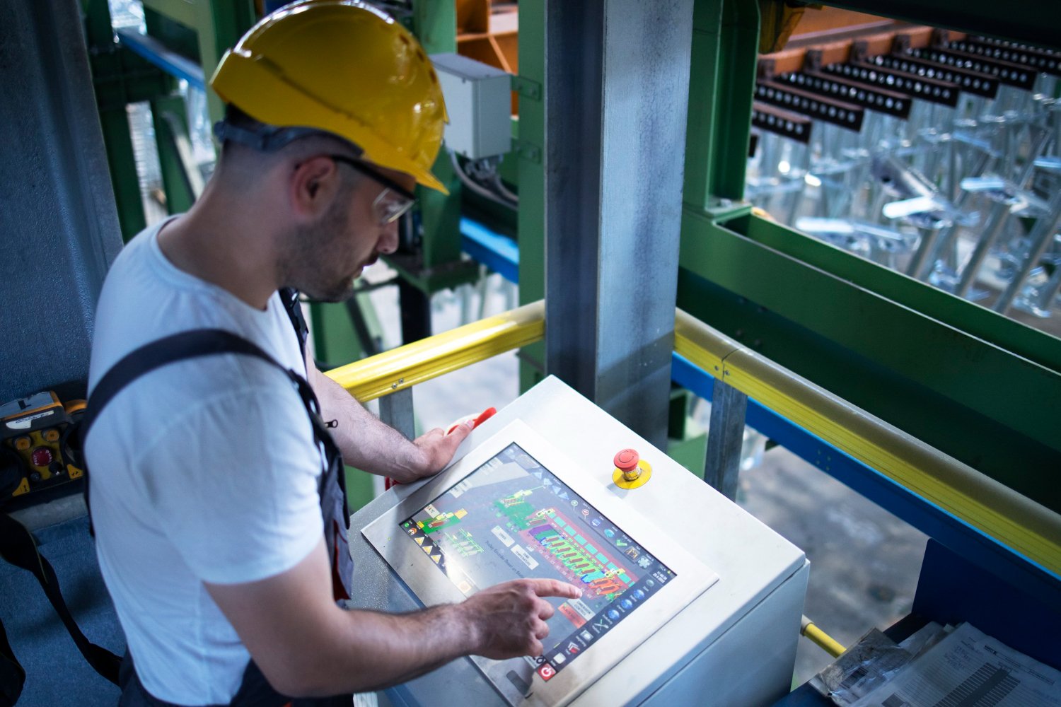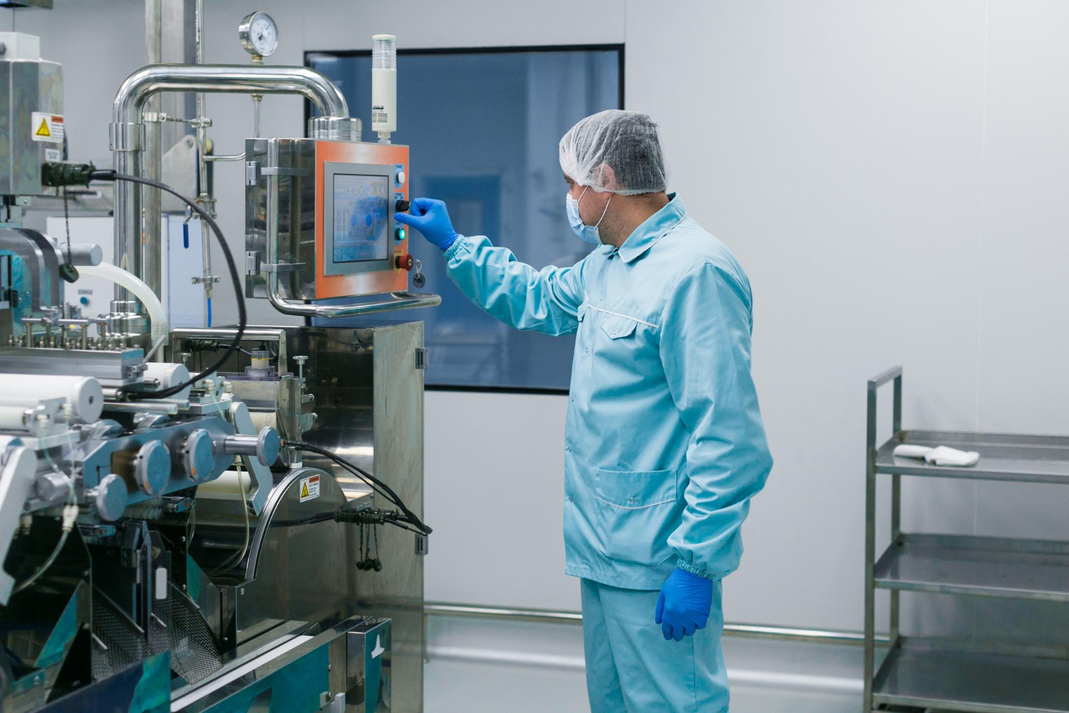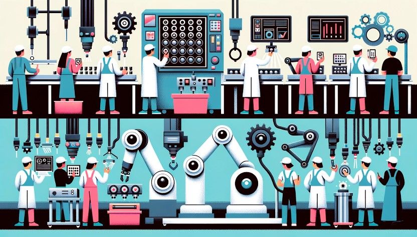
Whether computer vision works in manufacturing is mostly decided on the line, not in the model. A machine vision system is a chain: lighting, a camera or other imager, a processor, software, and output devices that turn each image into a pass/fail decision, a reject signal or position data for a robot. Its accuracy depends on how completely the defect set was defined, and conventional systems also need capture physics that yields simple contrast. Only after that does it matter whether the software uses hand-written rules or a trained network.
The factors that decide success are lighting and part presentation, how the reject decision reaches the PLC, the cost compared with manual inspection, and the accuracy a pilot loses when it moves from the lab bench to production. The light you can control and the defects you can define set the ceiling; the software only works underneath it.
How a machine vision system turns an image into a reject
The first step in automatic inspection is image acquisition, using cameras, lenses and lighting designed to give the differentiation the later processing needs. Processing then runs in stages: filters that modify the image, extraction of objects, extraction of data from those objects (measurements, code reads), and finally a comparison against target values that produces a pass/fail result. That result can trigger a mechanism that rejects the part or sounds an alarm. Other common outputs are position and orientation data for robot guidance.
Conventional machine vision depends on that “physics” phase producing simple differentiation, for example dark defects on a light part. A common reason applications were not doable was that this simple contrast could not be achieved. Deep learning removes the requirement and treats the object more as a human inspector would. Most of the decisions that follow come down to that one line, between problems that light and optics can turn into simple contrast and problems they cannot.
How a machine vision system differs from a custom computer vision build
Traditional machine vision runs on hand-coded rules: engineers set edge thresholds, blob sizes, pixel counts and pass/fail logic for each feature of the part. These systems are fast and repeatable. They work well on stable, high-volume parts where the defect set is known and the design is locked. If the part geometry, lighting or surface finish changes, the rule set often has to be rebuilt from scratch.
A custom computer vision system replaces hand-set rules with a model trained on images of the part. That model can handle defects that never produce clean contrast. Its accuracy still covers only the defects it was trained or programmed to look for: a system built to catch scratches will not flag a missing connector. Here, “machine vision” means packaged inspection hardware with configured software, and “custom computer vision” a system engineered around a trained model for one problem. The key differences between machine vision and computer vision are untangled in more depth elsewhere.
Is computer vision AI, and does the answer change how we buy it?
Only some of it is. A 2024 review of generative AI in industrial machine vision by Zhou and colleagues notes that traditional computer vision algorithms are still widely used, while machine learning has become central to current research. A thresholding or pattern-matching tool is classical image processing, not machine learning.
The procurement path does change with the answer. We would buy a rule-based system like equipment: specify it, configure it, validate it, and leave it alone until the part changes. A learned system is closer to a service with a lifecycle. Machine vision’s ongoing costs include maintenance, periodic retraining when a product or process changes, and engineering support. So the contract and the budget should say who owns the labelled data, who retrains the model and who decides when it needs retraining. If those questions are left out at purchase, they come back later as an unplanned cost.
Which defects push the decision toward learned computer vision versus rule-based machine vision?
Oxmaint, a vendor, positions rule-based vision for deterministic checks (dimensional measurement, barcode reading, presence/absence) and deep learning for subjective, variable defects such as scratches, texture anomalies and surface contamination. That split matches the physics argument: conventional vision needs simple contrast, and deep learning removes that requirement.
Some inspection cases remain challenging:
- Transparent and overlapping objects, parts imaged under dark-field or back light, parts whose normal appearance varies a lot, and extremely small defects. The MVTec AD 2 dataset was built around these challenging cases, which previous datasets had not considered.
- Inspection under changing light. MVTec AD 2 adds test scenarios with lighting changes specifically to check robustness under real-world distribution shift.
- Wire harnesses. A systematic review of vision for robotised wire-harness assembly found that the automotive industry has yet to find a vision solution that recognises harness components as robustly as humans do.
- Rare or novel defects. Humans handle novel situations better than machines, and manual inspection stays the sensible choice when a defect is so rare or unusual that training a model for it cannot be justified.
If your defect falls into one of those categories, we would treat feasibility as an open question until it has been tested on your own parts under your own lighting. The wider quality control review process for computer vision in manufacturing is where those test results feed in.
Lighting, fixturing and conveyor speed decide most inspections
Advanced Illumination’s guide to machine vision lighting says that no other part of vision system design has consistently caused more delay, cost overruns and general frustration than lighting. The same guide sets three acceptance criteria for any lighting design: maximise contrast on the features of interest, minimise contrast everywhere else, and provide some robustness. A design that meets only the first two can still work, but only if part size, shape, orientation and placement never vary and ambient light never gets in.
Which technique fits depends on the sample’s surface and composition. Geometry matters most for specular parts, and wavelength and filtering matter most for colour and transparency. Infrared penetrates polymers well, while blue light, which penetrates less, shows shallow surface features on black rubber or laser etchings. Some defects show up better under diffuse light and others under directional light. Ambient light can have a tremendous impact on inspections: overhead factory lights, sunlight, and even task lighting from neighbouring inspection stations. AWS’s guidance for its Lookout for Vision proof-of-concept kit makes the same point from the model side: daylight through windows changes the scene, and pose and lighting must match the training setup to avoid false anomalies.
Fixturing takes variation out before the camera sees the part. In one connector study from the wire-harness review, the parts were placed on a flat table so that height was constant and only yaw varied, which let the study process 2D grayscale images only.
Line conditions to pin down before choosing lights
Advanced Illumination’s checklist covers the conditions to settle first:
- Working volume: access for camera, lens and lights in 3D space, and minimum and maximum working distance and field of view.
- Part motion: stationary, moving or indexed, plus speeds, feeds and cycle time.
- Strobing: pulse rate, on-time and duty cycle.
- Vibration: continuous or shock.
- Presentation: whether orientation and position are consistent.
- Ambient light: any risk of contamination.
The guide’s advice is to test two or three light types first on the bench, then on the floor where possible. When the station is designed from scratch, the lighting should be settled first and the parts handling built around it.
Worked example: exposure time against conveyor speed
Motion blur happens when the part moves during exposure, and it grows with both part speed and exposure time. Vision-Doctor’s example uses a 120 mm part, a 5-megapixel camera with 2,464 pixels in the direction of travel, and a conveyor moving at 600 mm/s.
- Size of one pixel on the part: 120 mm ÷ 2,464 px ≈ 0.049 mm.
- Time the part takes to move one pixel: 0.049 mm ÷ 600 mm/s ≈ 0.000081 s, or about 81 µs.
- One pixel of blur therefore needs an exposure of roughly 0.08 ms. Vision-Doctor puts typical industrial exposure times at 0.1 to 20 ms, and says a blur of 0.5 to 2 pixels is invisible to the eye but still reduces measurement accuracy.
That is below the typical 0.1 to 20 ms range, so a one-pixel limit calls for more light, and light becomes the limiting resource: using dual polarisers to kill glare can cost up to 2½ f-stops, which Advanced Illumination flags as harmful in high-speed, light-starved inspections.
Which production constraints (latency, lighting, throughput) push the choice?
Throughput favours rule-based checks wherever the defect allows them. Oxmaint describes a hybrid in which a high-speed rule-based stage checks dimensions, presence and labels at full line speed, rejects obvious failures and passes borderline parts to a second, learned stage.
Latency is a hard limit, not a tuning parameter. In robotised assembly the vision system has to perceive the part fast enough for the next robot action, and the wire-harness review found processing time still a challenge against real production requirements. For a learned model we would measure inference time on the actual target hardware at line rate before committing, because a model that is accurate offline but misses the reject window is of no use on the line.
Oxmaint rates rule-based systems as highly sensitive to lighting and deep learning as more tolerant. The production study discussed below, however, shows deep-learning inspectors degrading badly when ambient lighting shifted under inadequate exposure settings. Being more tolerant of lighting changes does not make a system immune to them. Where you cannot control the light, neither approach is safe.
Wiring the reject decision into the PLC
On the line, the pass/fail decision triggers the reject mechanism or alarm. For Cognex In-Sight cameras, that link follows a documented procedure. For a Cognex In-Sight camera talking to a Rockwell ControLogix PLC over EtherNet/IP, the vendor’s documentation has you install the camera’s EDS file, configure RSLogix 5000 or Studio 5000 to recognise the camera, and select EtherNet/IP as the protocol in the camera’s industrial Ethernet settings. Switching from another protocol such as PROFINET may require a restart.
A custom computer vision system has to build that link itself, with the timing from trigger to actuator as a design item. We would also log every image with its prediction and confidence from the first day on the line. The 2024 continuous-training study logs every input with its prediction and calibrated confidence between retraining cycles. Where the station sits (inline or offline) and the hardware choices are covered in our piece on vision systems for manufacturing quality control and PLC integration.
Machine vision vs computer vision: which inspection approach fits my line?
The table below sums up the decision. Each row is a signal, not a verdict, and a line that splits across the rows is a candidate for Oxmaint’s hybrid design.
| Line condition | Points to rule-based machine vision | Points to learned computer vision |
|---|---|---|
| Defect type | Dimensions, presence/absence, codes and labels | Scratches, texture, contamination, cosmetic variation |
| Contrast | Lighting can make defects simply distinguishable | Simple differentiation is not achievable |
| Design stability | Locked geometry and finish | Normal variation in appearance that rules cannot list; when the design is still changing, manual inspection keeps the advantage |
| Defect set | Known and fully specifiable | Definable by examples rather than thresholds |
| Lighting control | Controlled and consistent | Less controlled, but matching the training setup |
| Speed | Full line speed | Fits the inference budget measured at line rate |
When does a Cognex- or Keyence-style system beat a custom CV deployment?
A packaged smart-camera system wins when the job is measurement, presence or code reading on a locked design under controllable light. In those conditions the rule set stays valid and, for cameras such as Cognex In-Sight, the PLC interface follows a documented procedure. Building a custom model for that kind of job adds a lifecycle without adding capability.
Custom computer vision earns its cost when the defect will not reduce to simple contrast. TechnoLynx engineers this custom side for manufacturers: learned inspection models, the data and retraining loop behind them, and their integration into the line, through its AI engineering for manufacturing and automotive work.
That work does not suit every line. If the requirement is a barcode read or a gauging check on a stable part, a vision vendor or its integrator is the more direct route. If the design is still changing, manual inspection is the honest answer until it settles.
How much does a vision inspection system cost, machine vision versus custom computer vision?
Vision moves cost to the front of a project. The investment goes into cameras and optics, lighting and fixturing, integration with existing controls, and software development or model training. After that come maintenance, retraining when the product changes, and engineering support. Capital cost varies widely with part geometry, defect type, line speed and integration needs, so a scoped figure for your own application is the only reliable comparison.
Published figures exist but are indicative at best. A3 (the Association for Advancing Automation) puts the average system at about $35K including hardware, software, application engineering and integration, in its cost-justification guidance. Oxmaint describes a $48K rule-based station checking hole positions on brake brackets, with a claimed payback of 1.5 months. That is a vendor’s account of one plant, not a benchmark. Neither figure is for a custom deep-learning system, whose costs include model training and retraining.
A3’s method for comparing vision with manual inspection works line by line:
- Labour: A3’s example assumes inspection labour falls to about 10% of the manual level.
- Scrap and rework: the example assumes rejects fall to about 20% of the current level, and notes that 100% inspection can flag trends before they produce rejects.
- Data quality: measurements are always taken the same way, with no transcription errors.
- Process control: inspection data can show process conditions drifting toward rejects.
Those percentages are A3’s assumptions for illustration. Replace them with your own figures.
Manual inspection is itself imperfect. The Sandia National Laboratories literature review (See, 2012) cites Swain and Guttmann’s 1983 estimate of a minimum human error rate of about 1 in 1,000 for simple accept/reject tasks. It also notes that error rates of 20% to 30% are frequently quoted across inspection tasks, and that 100% inspection still misses defects. The same review cites Drury and Fox (1975) for detection deteriorating by up to 40% within 30 minutes. Sciotex, a vendor, puts human misses at up to 40% and vision accuracy at 97% to 99%, but only on the defects the system was built to find. That qualifier matters more than the headline figures.
Vision tends to win on total cost when the design is stable, the defect set can be defined and escaped defects are expensive. Manual inspection remains a sensible choice when designs change, volumes are low, part numbers change constantly or first-article judgement is needed. Price both failure directions in the model. Signal detection theory implies that near-perfect detection comes only with more false alarms, and for many inspection tasks a missed defect costs far more than reworking a good part.
Who maintains the system when the team that built it moves on?
A rule-based system’s logic is explicit: hand-coded thresholds, blob sizes and pass/fail rules. Its weakness is sensitivity to change. A change in geometry, lighting or finish can mean rebuilding the rule set.
Continuous training of a learned system needs fresh labelled samples from the original distribution, and retraining on self-generated labels can degrade performance without anyone noticing. The authors note that retraining on drifted data, even with correct labels, does not guarantee a working model, and they treat such data as unreliable because it can cause catastrophic forgetting. The 2024 study’s own approach needed domain experts to define realistic augmentations during setup.
The handover package therefore needs more than model weights. We would expect it to include the training and validation images, written defect definitions with examples, the capture specification (lighting, pose, exposure) and the retraining procedure. The Sandia review found that unclear definitions led inspectors to form personal criteria that drifted over time, and labellers on a model project are inspectors in all but name.
Why computer vision pilots lose accuracy on the production line
A study of two deep-learning inspection systems, one for printed wooden sticks and one for glass bottles, shows the effect. Validation F1 was 93.2% and 93.3%. On production data it fell to 45.7% for the stick prints and 76.6% for the bottles. The causes were changes in the production environment. Ambient lighting on the premises shifted the data because the camera exposure settings were inadequate, and a new open-mark defect appeared on the bottles, which pushed the model’s predictions close to random. On the stick line, a slightly damaged ink dispatcher in the printer produced smudged prints, a defect type the model had never seen.
The failure was silent. False acceptance rose fivefold for the sticks and tenfold for the bottles, while rejection rates stayed low and stable. Neural networks produce an output for any well-formed input, even one outside the domain they were trained for. The authors’ filtered retraining raised production F1 on the stick line to 59.7%.
The wire-harness review points the same way. The research it covered remained laboratory experiments, and individual studies named complex backgrounds and varying illumination as causes of failure. The Sandia review notes the human equivalent: a separate test gives an upper bound on performance, because tests are not representative of normal working conditions.
How should a manufacturer size a computer vision pilot before scaling it across lines?
Size a pilot by the conditions it covers, not by the number of images. AWS’s Lookout for Vision documentation sets a low minimum. To start training a classification model it needs at least 20 normal and 10 anomalous images, and for segmentation at least 20 images of each anomaly type plus 20 normal ones. It recommends more than the minimum for a higher-quality model, unique images, and consistent camera position, lighting and pose. Those numbers are the minimum to start training. They say nothing about whether the model will survive a night shift or a sunny afternoon.
Augmentation is one way to stretch a small dataset. In one study cited by the wire-harness review, elastic-transform augmentation improved performance on small datasets. Even the AWS and Basler proof-of-concept kit expects hardware and software changes before production and offers a gap analysis after the pilot.
A pilot sequence that survives the move to production
- Write the defect definitions with image examples, and put a cost on an escaped defect and on a false reject.
- Settle lighting and presentation on the bench, then repeat the test on the floor.
- Collect production images across shifts, daylight changes, material lots and changeovers.
- Run the system beside the existing inspection, logging every image with its prediction and confidence.
- Report false accepts separately: in the study they rose while rejection rates stayed stable.
- Assign drift monitoring and retraining ownership before a second line is added.
Treat each new line as a new lighting environment with its own ambient sources, not a copy of the first. A pilot that passed under one set of overhead lights has proved that the method works, not that the next line will.
FAQ
Is computer vision obsolete?
No. The 2024 review by Zhou and colleagues notes that traditional computer vision algorithms remain widely used, while machine learning has become central to current research.