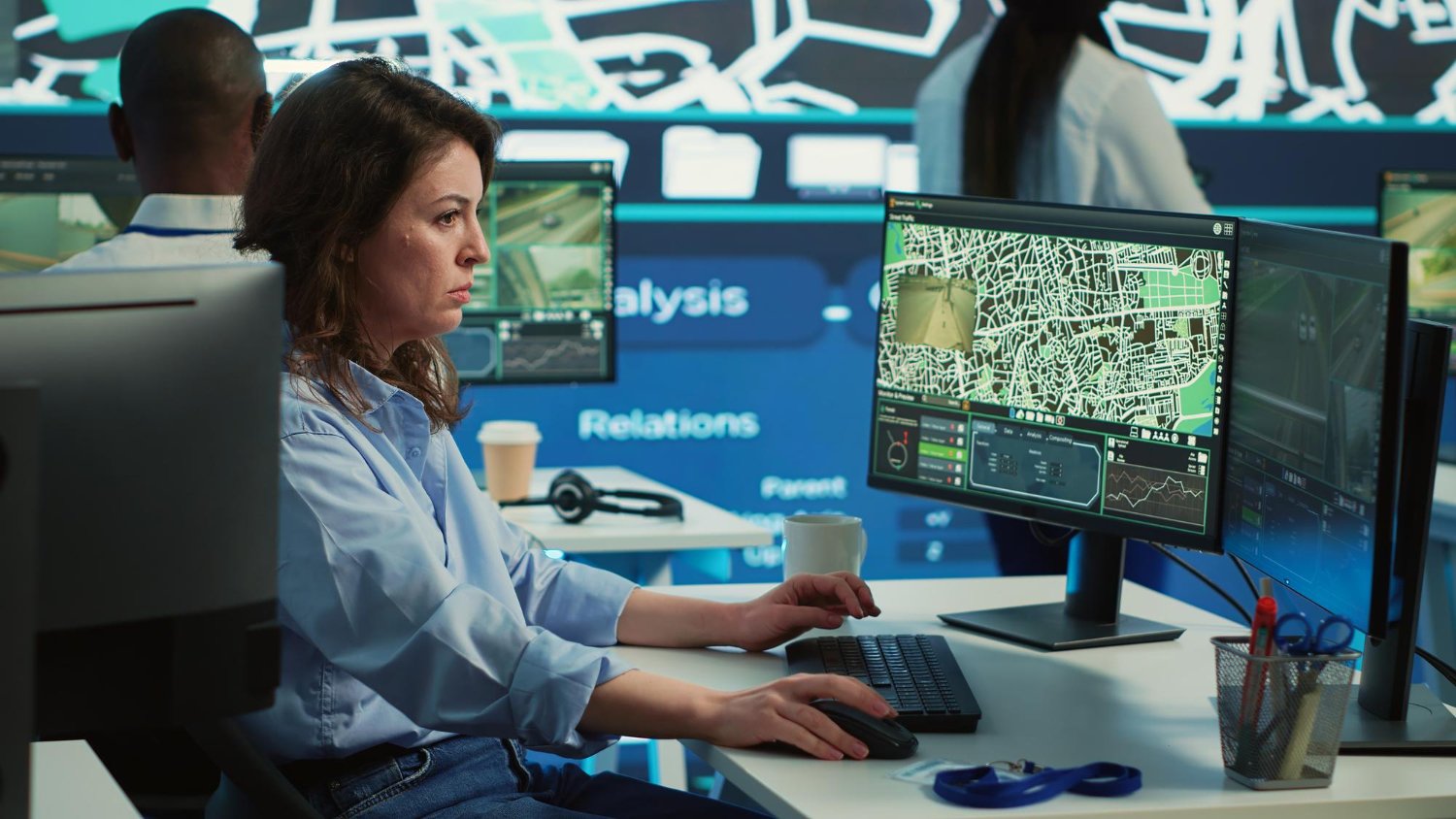
Search “deep learning self driving car” and you get a clean diagram: cameras and lidar feed a neural network, the network outputs detections, the car drives. The diagram is not wrong. It is just the part that never fails. The interesting question — the one that decides whether a perception stack ships or stays in validation — is what the model does when the road stops looking like the training set.

A deep learning perception model in a self-driving car is, at its core, a function that maps raw sensor data to a structured understanding of the scene: where the other cars are, where the lane markings run, whether that shape at the edge of the frame is a pedestrian or a reflection. The function is learned, not written. And learned functions have a property that hand-written code does not: they are confident in exactly the places they have seen before, and unpredictable everywhere else. Understanding how deep learning perception works in practice means understanding that property, because it is where real roads break real models.

How does a deep learning self-driving car work in practice?

The pipeline has three broad stages, and each is more fragile than the diagram suggests.

First, sensing. Cameras produce dense pixel arrays; lidar produces sparse point clouds; radar produces range-and-velocity returns. None of these arrive in a form a neural network can consume directly — they are calibrated, time-synchronised, and projected into a common reference frame before anything learns from them. If the calibration is wrong, the network learns from a distorted picture of the world, and no amount of training corrects a systematic geometric error. This is why camera extrinsic calibration belongs in the safety evidence, not just the engineering backlog.

Second, perception. This is where the deep learning lives. Convolutional backbones and transformer-based detectors — architectures in the lineage of YOLO, DETR, and bird’s-eye-view models like BEVDet — take the processed sensor data and emit detections: bounding boxes, segmentation masks, tracked objects, lane geometry. A modern stack rarely uses one model; it uses several, each specialised, feeding a fusion layer.

Third, decision and control, which is downstream of perception and depends entirely on it being right. A planner that receives a confident, wrong detection has no way to know it is wrong. Perception is the layer that gets to be uncertain; everything after it inherits whatever perception decided.

The reason the naive reading of that pipeline is dangerous is that it treats the neural network as a solved box. In practice, the network is the component whose behaviour you understand least precisely, because its behaviour is defined by data you can only partially characterise.

What sensors feed the network, and how does it turn them into detections?

The inputs are heterogeneous by design. Camera gives semantics — colour, texture, the difference between a truck and a billboard. Lidar gives geometry — precise range, unaffected by lighting. Radar gives velocity and works through rain and fog where cameras degrade. A perception model that fuses all three is more robust than any single modality, but fusion is also where subtle failures hide: if the camera and lidar disagree about where an object is, the fusion layer has to arbitrate, and the arbitration rule is itself learned or tuned against a particular data distribution.

Turning raw sensor data into detections is a sequence of learned transformations. A camera-based detector, for example, passes the image through a backbone that extracts features at multiple scales, then a detection head that proposes and classifies regions. The difference between architectures — whether you use a region-proposal approach in the R-CNN family or a single-shot detector — changes latency, small-object behaviour, and the shape of the failures, but not the fundamental fact that the model outputs a probability distribution over classes and locations. That distribution is calibrated to the training data. Move the input distribution and the probabilities stop meaning what they claimed to mean.

Why does high benchmark accuracy not prove a model is ready for real roads?

Here is the misconception worth naming directly: a high benchmark score is a claim about a dataset, not about the world. When a perception model reports strong mean average precision on a public benchmark, that number describes performance on the distribution the benchmark sampled — the weather, the geographies, the sensor rigs, the object frequencies that dataset happened to contain. A real road is a different distribution, and the gap between the two is not a rounding error.

The distinction between reported and operational accuracy is one we return to often, because it is the single most common source of over-confidence in automotive perception. It is worth being precise about what a metric proves and what it merely asserts — the difference between what each performance metric actually proves and what a stakeholder reads into it.

The claim that matters:

Benchmark accuracy measures a model against the distribution the benchmark sampled. Road-readiness depends on the model’s behaviour on the production driving distribution — the two coincide only to the extent the benchmark represents the road, which is rarely and never completely.

A quick diagnostic: is your benchmark score telling you the truth?

Question	If “no” or “unsure”	What it means
Was the benchmark collected on your sensor rig and mounting geometry?	Score does not transfer directly	Calibration and viewpoint shift the input distribution
Does the benchmark contain your operating weather and lighting range?	Long-tail conditions untested	Model may collapse on rare-but-real scenarios
Are rare object classes represented at real-world frequency?	Tail classes under-measured	High mAP can hide poor tail-class recall
Is the failure rate reported per scenario class, not just aggregate?	Aggregate hides the tail	One good number masks several bad ones
Has the model been audited against a divergence set, not just the test split?	No robustness signal	You know the average, not the worst case

If more than one row lands on the wrong side, the benchmark number is a measurement of the dataset, not a prediction about the road.

Where do deep learning perception models fail — and why is the long tail the hard part?

The failures cluster in the long tail: the rare scenario, the unusual object, the lighting condition that appears once in ten thousand frames. A model trained on millions of examples learns the common cases with remarkable precision. The problem is that road safety is not decided by the common cases. It is decided by the rare ones — the pedestrian in an unusual pose, the debris in the lane, the emergency vehicle at night in the rain. These are, by construction, under-represented in any training set, because they are rare in the world.

This creates a structural asymmetry. Adding more common-case data improves the benchmark and barely touches the failure modes that actually cause incidents. The perception failure modes that survive benchmarks — the ones that show up only when you exercise the model against a deliberately divergent distribution — are a category worth studying on their own; we have written about the perception failure modes that survive benchmarks precisely because they are invisible to the metrics teams usually track.

Weather, lighting, and sensor mounting variance are the three axes along which the production distribution most reliably diverges from training data. Rain scatters lidar and blurs cameras. Low sun saturates sensors and casts long shadows the model may read as objects. A camera mounted two centimetres from its calibrated position — a repair, a manufacturing tolerance, a thermal shift — changes the geometric projection the model learned to interpret. Each of these changes what the model sees, and a model only generalises across the variance it was trained and validated against. Observed across automotive perception work, the conditions that matter most are almost never the ones the initial dataset emphasised; this is an observed pattern from field validation, not a benchmarked rate.

Common cases versus the production driving distribution

There is a meaningful difference between a model that learned the common cases and one that generalises to the production driving distribution. The first is easy to build and easy to benchmark well. The second requires knowing what the production distribution actually contains — which weather, which geographies, which edge classes, which sensor configurations — and validating against it deliberately.

The honest position is that no model fully generalises to a distribution you have not characterised. You cannot validate against edge cases you have not enumerated, and you cannot enumerate them from the training set alone, because the training set is where the common cases live. This is why understanding how the model learns is the on-ramp to understanding how it must be tested: the learning process tells you exactly where to be suspicious.

For a fuller treatment of how the same learned behaviour looks from inside the production perception stack — where fusion, tracking, and temporal consistency enter the picture — the companion piece on how perception models actually work in production covers the deployment-side detail this explainer deliberately leaves out.

Where does a robustness audit fit relative to how the model was built?

Once you accept that benchmark accuracy is a distributional claim, the release decision changes shape. The question is no longer “what is the mAP?” but “what is the long-tail failure rate per scenario class, and how long does validation take to expose it?” These are the measurable outcomes that connect an abstract architecture to an actual go/no-go decision: long-tail failure rate per scenario class, validation pass-through time, and post-release surprise rate.

A robustness audit sits exactly at the seam between how the model was built and whether it can ship. It takes the learned behaviour described in this article and stress-tests it as a perception workload against the production driving distribution — deliberately feeding the model the divergent conditions the benchmark under-sampled, and measuring where the learned features break. The reliability-audit methodology treats the perception model as a versioned artifact whose behaviour under stress must be recorded, not assumed. Our broader computer vision engineering practice is built around this distinction: the value is not in pushing benchmark points, but in knowing where the learned features stop being trustworthy.

Knowing where a model’s learned features break lets a team target data collection and audit design at the failures that matter, instead of chasing benchmark improvements that never translate to road performance. That redirection — from average-case optimisation to tail-case validation — is the practical payoff of understanding how deep learning perception actually works.

FAQ

How does a deep learning self-driving car work?

A deep learning self-driving car uses learned neural networks to map raw sensor data — camera, lidar, radar — into a structured understanding of the scene, which downstream planning and control then act on. In practice this means the perception layer is a learned function that is confident where it has seen data before and unpredictable elsewhere, so the behaviour that matters most is what it does outside its training distribution.

What sensors and inputs feed a deep learning perception stack, and how does the network turn them into detections?

Cameras provide semantics, lidar provides precise geometry, and radar provides velocity and works through rain and fog. Each is calibrated, time-synchronised, and projected into a common frame, then passed through learned backbones and detection heads that output a probability distribution over object classes and locations — a distribution calibrated to the training data.

Why does high benchmark accuracy not prove a perception model is ready for real roads?

A benchmark score is a claim about a dataset, not the world: it describes performance on the distribution the benchmark sampled. Road-readiness depends on behaviour on the production driving distribution, and the two coincide only to the extent the benchmark represents the actual road — rarely, and never completely.

Where do deep learning perception models fail — and why is the long tail the hard part?

Failures cluster in the long tail: rare scenarios, unusual objects, and lighting conditions that appear in a tiny fraction of frames. A model learns common cases beautifully but road safety is decided by rare ones, and adding more common-case data improves the benchmark while barely touching the failure modes that cause incidents.

How do weather, lighting, and sensor mounting variance change what the model actually sees?

Rain scatters lidar and blurs cameras, low sun saturates sensors and casts shadows the model may read as objects, and a camera even slightly off its calibrated mounting changes the geometric projection the model learned to interpret. Each shifts the input distribution, and a model only generalises across the variance it was trained and validated against.

What is the difference between a model that learned the common cases and one that generalises to the production driving distribution?

A model that learned the common cases is easy to build and benchmarks well; a model that generalises to the production driving distribution requires knowing what that distribution actually contains and validating against it deliberately. No model fully generalises to a distribution you have not characterised, because you cannot validate edge cases you have not enumerated.

Where does a robustness audit fit relative to how the perception model was built?

A robustness audit sits at the seam between how the model was built and whether it can ship. It takes the learned behaviour and stress-tests it against the production driving distribution — feeding the divergent conditions the benchmark under-sampled and measuring where the learned features break — turning an abstract architecture into a defensible release decision.

When the next unusual scenario appears on the road, the model will respond the way its training distribution taught it to — the only open question is whether you measured that response before the road did.