A precision decision is not a setting you flip. It is a commitment with a re-entry cost, and the cost is almost never paid at the moment of the decision — it is paid at the next migration, when someone asks whether the deployed model can run somewhere else.
The question usually arrives in a mundane form. A new accelerator generation lands and procurement wants a comparison. A customer requires on-premise deployment on hardware you did not choose. A model upgrade arrives and the vendor ships weights in a format your serving path never anticipated. In each case the technical question is the same: what does it cost us to change numerical regime now that the system is in production?
Teams that quantised carefully can usually answer in days. Teams that quantised opportunistically often cannot answer at all, because the calibration data is gone, the tolerance that was considered acceptable was never written down, and nobody remembers which layers were kept in higher precision or why.
The distinction that matters: precision as a setting versus precision as a commitment
Teams run into trouble when they treat precision as a configuration parameter they can toggle between deployments without consequence. For a weight-only INT8 conversion of a small vision model with a stored calibration set, that framing is roughly accurate. The conversion is cheap, the reversal is cheap, and the evidence needed to justify either is small.
It stops being accurate the moment the precision decision propagates outward. A stack built around one numerical format tends to accumulate dependencies on it: fused kernels that only exist for that format, a serving configuration tuned to its memory footprint, capacity planning that assumes its throughput, and — most consequentially — an accuracy baseline that was established after quantisation rather than before. Once the baseline is post-quantisation, the team has lost the reference point it would need to evaluate any alternative.
Over-specialising a stack to a single numerical format narrows the set of models, runtimes, and devices that remain viable later — and that narrowing is invisible until something forces the comparison.
This is not an argument for staying in FP32. Lower precision is frequently the correct engineering decision, and refusing it to preserve theoretical flexibility is its own failure. The argument is narrower: the decision has a second cost column, it is rarely estimated, and it is estimable.
Which precision decisions are reversible and which are one-way doors?
Evidence quality—calibration data, pre-quantization checkpoints, and evaluation harnesses—determines whether you can reverse course, not the file format you chose. The same INT8 target can be cheaply reversible in one deployment and effectively one-way in another. The differentiator is what was preserved.
| Decision shape | Re-entry cost | Why |
|---|---|---|
| Post-training weight-only quantisation, calibration set archived, FP baseline retained | Low — re-export and re-validate | The higher-precision artefact still exists; reversal is a build step |
| Post-training quantisation with activation calibration, calibration data archived | Moderate — recalibrate, revalidate against retained baseline | Recalibration is mechanical if the data survived; validation is the real work |
| Quantisation-aware training or fine-tuning at the target precision | High — retraining, not re-export | The deployed weights are not a lossy view of an FP checkpoint; they are a different checkpoint |
| Sparsity or structured pruning combined with a precision commitment | High — coupled decisions must be unwound together | The two are entangled; reversing one changes the accuracy premise of the other |
| Any of the above with calibration data or tolerance thresholds lost | Effectively a rebuild | The decision must be re-derived from scratch, including the acceptance criteria |
Evidence class for this table: observed-pattern — it reflects how quantisation reversals have gone in engagements we have been close to, not a benchmarked migration-cost model. Your ordering may differ; the structural point is that the bottom two rows are qualitatively different from the top two, and teams routinely land in them without noticing.
The last row deserves emphasis because it is the most common and the most avoidable. Losing the calibration set converts a moderate reversal into a rebuild. Losing the written tolerance — the statement of what accuracy degradation was accepted, on which evaluation set, judged by whom — converts a revisable decision into a re-litigated one, which in practice means it does not get revisited at all.
The re-entry cost decomposes into three layers
“Hard to revert” conflates three distinct expenses: re-quantizing from scratch, re-running evaluation suites, and explaining latency changes to stakeholders.
Recalibration is the mechanical layer. Regenerate calibration statistics, re-run the export, rebuild the engine. With TensorRT this is a matter of re-running the builder against a stored calibration cache or the original representative dataset; with ONNX Runtime’s quantisation tooling it is similar. If the inputs survived, this layer is measured in hours.
Revalidation is the expensive layer. The accuracy evidence that justified the original precision must be regenerated for the new regime, on the same evaluation set, against the same tolerance. For a classifier with a stable held-out set this is tractable. For a generative model where the acceptance criterion involved human judgement or a task-specific eval harness, revalidation can dominate the entire migration — and it does not shrink just because the change is back toward higher precision. Raising precision still changes outputs, and outputs that changed require re-approval in any regulated or contractual setting.
Rebuild is the layer nobody budgets for. If the deployed weights were produced by quantisation-aware fine-tuning, or if the serving path assumes a format-specific kernel — a fused attention implementation available in one precision but not another, or an FP8 path in a runtime whose FP16 path was never exercised — then reversal means producing a new artefact through a new pipeline. Quantifying this as a general figure is not possible; it depends on whether the training data, recipe, and compute are still available.
The useful discipline is to name which layer you are in before estimating. A team that believes it is in recalibration and is actually in rebuild will miss its migration window by a wide margin.
How lock-in shows up as a hardware and runtime constraint
An INT4 checkpoint cannot be upcast to recover FP16 fidelity, unlike ONNX graphs that convert across runtimes with predictable semantics. FP16 and BF16 are broadly supported across contemporary accelerators; INT8 is widely supported but with meaningful differences in how activation ranges and per-channel scaling are handled; FP8 and FP4 support varies by hardware generation and by which runtime paths have been implemented, per the vendors’ own published documentation rather than any measurement of ours.
The practical consequence is that a stack committed to a narrow format has fewer devices it can be fairly compared on. That is the point at which the lock-in becomes visible: someone requests a cross-device comparison and discovers that half the candidate devices cannot run the deployed artefact at all, so the comparison has to be run on a re-derived artefact that no longer represents the production system. The measurement becomes a proxy for a system that does not exist.
This is precisely why a per-precision result across devices, produced before the commitment, is worth more than the same result produced after it. Reading a device’s numbers only at the precision you have already chosen tells you what you have; reading them across the precisions the device supports tells you what you are giving up. Our work on what precision formats a device actually supports, as distinct from what its spec sheet lists covers the support-matrix side of this; the measurement of the precision-to-accuracy trade-off itself covers what the current choice costs today. Neither answers the optionality question, which is what this page is for. The broader methodology sits on the LynxBenchAI benchmarking methodology page.
There is a related asymmetry worth naming: throughput gains from lower precision are usually measured at the moment of adoption, while the constraint on future device choice is paid years later by a different team. That timing mismatch is why the second cost column so rarely appears in the original decision memo.
What to record at the moment of the decision
Storing the original high-precision checkpoint and the calibration dataset takes five minutes during the initial export and becomes archaeologically difficult six months later. Recording the calibration data, tolerances, and evidence behind a precision decision is what makes the decision revisable rather than re-derivable.
A minimum record, in our view:
- The higher-precision reference artefact — the FP16 or FP32 checkpoint the quantised model was derived from, retained as a build input rather than deleted after export.
- The calibration dataset or cache, versioned alongside the model, with a note on how the representative samples were selected.
- The accepted tolerance, stated as a number on a named evaluation set: which metric, what degradation was accepted, and who accepted it.
- The per-layer or per-module exceptions — which parts of the network were held at higher precision, and the reason. This is the detail most often lost, and the one that makes a reversal reproducible.
- The runtime and version the export was validated against, because a quantised artefact’s behaviour is a property of the executor, not of the weights alone.
- What was not tested — the precisions considered and skipped, so the next team does not redo the elimination.
Six bullet points in a repository is the difference between a two-week migration and a two-quarter one. We treat the absence of this record as a finding in its own right when reviewing an inference stack, because it converts every future precision question into a research project.
A worked estimate, with its assumptions stated
Consider that scenario: a 7B model at INT8 weight-only quantization, calibrated on 512 samples, with the FP16 source checkpoint archived and versioned alongside the deployment artifact. A new deployment target requires BF16.
Under those assumptions the work is: re-export from the retained checkpoint, rebuild the serving engine, and re-run the existing eval harness against the recorded tolerance. There is no recalibration step, because weight-only quantisation of a retained checkpoint is a build transformation. The dominant cost is revalidation, and its size is set by the eval harness, not by the precision change.
Change one assumption — the model was fine-tuned at INT8 rather than converted — and the same request becomes a training job with an uncertain schedule. Change another — the calibration set was never versioned — and even the INT8 path cannot be reproduced, so the comparison baseline has to be rebuilt before the migration can start. This is an illustrative decomposition rather than a measured one; the point is that the assumptions, not the formats, determine the cost.
FAQ
What does committing a deployed system to one precision regime foreclose later?
It narrows the set of models, runtimes, and devices that can run the production artefact without rework. Formats differ in how widely they are supported across accelerator generations and in which runtime paths have been implemented, so a narrow commitment reduces the number of candidates a future comparison can legitimately include. The foreclosure is usually invisible until a migration or a cross-device comparison forces it into view.
Why is over-specialising a stack to a single numerical format a risk rather than an achievement?
Because the surrounding stack accumulates dependencies on the format — format-specific fused kernels, a capacity plan built on its footprint, and an accuracy baseline established after quantisation rather than before. Once the baseline is post-quantisation, the reference point needed to evaluate any alternative is gone. The throughput gain is real; it is simply not the whole ledger.
What is the actual re-entry cost of changing precision after a system is in production — recalibration, revalidation, or rebuild?
It decomposes into all three, and naming which one you are in comes first. Recalibration is mechanical — hours, if the calibration inputs survived. Revalidation means regenerating the accuracy evidence against the recorded tolerance and is often the dominant cost. Rebuild means producing a new artefact through a new pipeline, which is where quantisation-aware training lands; teams that assume recalibration and are actually in rebuild miss their migration window.
What evidence has to survive for a precision decision to stay reversible?
The higher-precision checkpoint, the calibration data, and the written accuracy tolerance the decision was signed off against. With all three retained, post-training weight-only quantisation reverses as a build step. Quantisation-aware training, and precision decisions entangled with sparsity or pruning, stay expensive even with the evidence intact, because the deployed weights are a distinct checkpoint rather than a lossy view of one. Any decision whose calibration data or written tolerance was lost is effectively a rebuild regardless of the format involved.
How does precision lock-in constrain a later migration to different hardware or a different runtime?
A quantised artefact’s behaviour is a property of the executor — hardware plus software stack — not of the weights alone, so moving either end can invalidate the validation that justified the original choice. When candidate devices cannot run the deployed artefact at all, the comparison has to be run on a re-derived artefact that no longer represents production, which turns the measurement into a proxy.
What should a team record at the time of a precision decision so that the decision can be revisited rather than re-derived from scratch?
The retained higher-precision checkpoint, the versioned calibration dataset, the accepted tolerance stated as a number on a named evaluation set, the per-layer precision exceptions and their reasons, the runtime version the export was validated against, and the precisions considered and skipped. This is a short record at decision time and close to unreconstructable afterwards.
Which downsides of a quantization decision are lock-in costs rather than accuracy costs, and why do they usually surface only at the next migration?
The narrowing of viable devices and runtimes, the loss of a pre-quantisation accuracy baseline, and the cost of regenerating validation evidence for any future regime are all lock-in costs — they are unaffected by how well the model scored after quantisation. They surface at the next migration because that is the first moment anyone asks the system to run somewhere it was not built for, and by then the original decision’s evidence is often gone.
A trade-off you can no longer measure has stopped being a choice
Choose instead how much optionality to preserve when selecting a precision for production. It is whether you can still read the trade-off from evidence after the commitment is made — whether a per-precision result across the devices you might plausibly move to exists in your records, or whether it will have to be re-derived under migration pressure from an artefact that no longer has a reference point. Precision is a first-class trade-off, and a trade-off you can no longer measure has quietly stopped being a choice.