An offline video inference pipeline for recorded footage runs decode, preprocessing, batched detection, tracking with re-identification, post-processing and output. In a published optimisation study of a multi-camera analytics pipeline, the bottlenecks came from scheduling, data flow and component interactions, not only from model inference; batching gains stopped at a certain batch size; and CPU-bound tracking and post-processing capped what parallelism could add. Once the pipeline is sized, the same replay harness can check multi-camera identity tracking without relabelling everything. You do that with stratified samples, a full set of tracking metrics and small labelled sets, and you take the acceptance thresholds from the workflow downstream, not from a universal number.
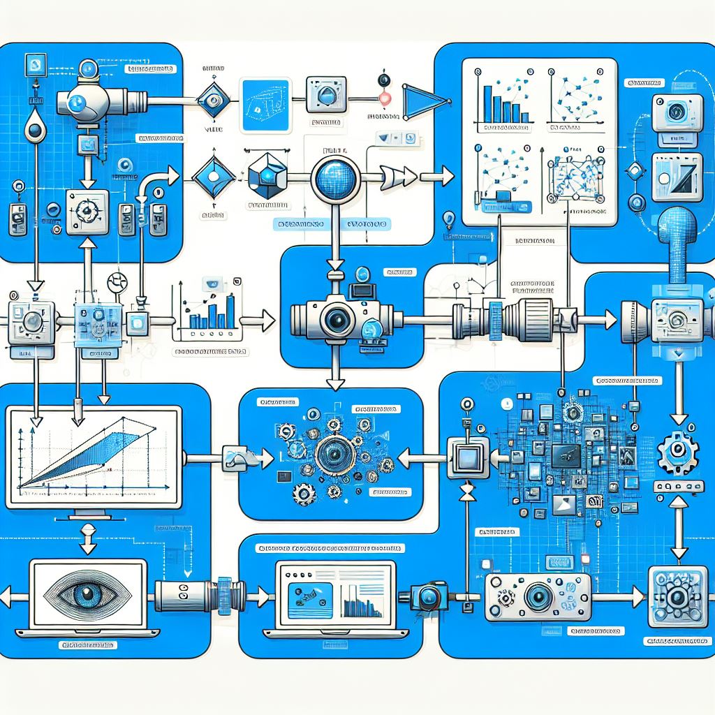
Stages of an offline video inference pipeline
The run order:
- Demux and decode. Compressed video is turned into frames. On NVIDIA GPUs this can run on NVDEC, the hardware decoder, which leaves the graphics engine and CPU free for other work and decodes much faster than real time.
- Preprocessing. Frames are resized, converted to the colour format the network expects, scaled and transposed to NCHW or NHWC.
- Batching. Frames from several sources are gathered into one batch for the GPU. In DeepStream the stream multiplexer (nvstreammux) does this.
- Detection inference. The model runs through a backend such as TensorRT or Triton Inference Server.
- Tracking. A detection-and-association tracker has four blocks: a detector, an embedding head that produces appearance descriptors, a motion predictor such as a Kalman filter, and an association module that solves the matching.
- Re-identification. A TensorRT network turns each detected object into a feature vector. The tracker uses these vectors to associate objects from frame to frame and to re-associate targets it has lost.
- Post-processing and output. Track initiation, termination and re-ID run here. The DeepStream tracker can also write per-frame results in a modified KITTI format and dump Re-ID features to text files.
The pipeline is only as fast as its slowest stage. Post-processing is easy to underrate: in the farm-video study, connected component analysis and bounding-box extraction stayed CPU-bound after detection had been accelerated, and adding parallel jobs just raised CPU load until the speedup levelled off.
Keeping one GPU busy: batching decode and inference together
Batching raises GPU efficiency. It has a ceiling, and on your own pipeline you find that ceiling by measuring. In the farm-video study, batch sizes from 1 up to 16 cut inference time per frame from about 6.6 ms to 2 ms, and GPU memory rose to a peak of 2301 MiB. Above batch 16, time per frame went up again because of memory pressure.
Combining batching with process-level parallelism did not simply add the two gains. In the same study, the original non-batched, single-process detection took 36 seconds. Batched inference brought that down to 23 seconds, but adding chunk-based multiprocessing on top gave 25 seconds, which the authors attribute to memory contention from larger GPU workloads. Our view is that you should tune batch size and process count together, on the target GPU, and never assume the best setting for one is still best once you change the other.
CPU-based decoding is another bottleneck to check. A vLLM write-up reported that large workloads had bottlenecked on CPU utilisation before 4 GPUs, and that at 8xH100 GPU decoding gave more than double the throughput of the CPU decoder. NVDEC capacity is set per engine: NVIDIA’s application note says a single decode session cannot go faster than one NVDEC engine, however many engines the GPU has. So you only get the aggregate throughput by running several decode sessions at once. FFmpeg can decode several inputs concurrently in one process, with one thread per decode and a shared CUDA context.
Three other decode-side choices appear in the sources:
- Prefetching. PyNvVideoCodec’s ThreadedDecoder decodes on a background thread so decode latency is hidden behind inference. NVIDIA recommends a prefetch buffer of 2 to 3 times the batch size.
- Selective decode. OpenCV’s
grab()moves the stream forward without decoding, andretrieve()decodes only the frames you will actually process. - Resolution and codec. For H.264, dropping from 1080p to 720p kept accuracy and cut decoding latency by more than half. MJPEG decoded fastest, but its artefacts slightly reduced detection robustness in low-light or occluded regions.
The tracker as the hidden bottleneck
A larger batch does not always raise GPU utilisation. NVIDIA’s VSS documentation notes that on GPUs such as the H100, a bigger batch may not raise utilisation in proportion, because the low-level tracker processes the whole batch on a single CPU thread. The fix is to enable sub-batches, which split the batch across parallel tracker instances. For 24 streams the documentation gives sub-batches=8:8:8 as an example. The DeepStream tracker guide says the best split has to be found by experiment: start with one batch and keep splitting it while comparing utilisation and performance, because every extra sub-batch adds overhead. Setting cudaDeviceScheduleBlockingSync with sub-batches enabled cuts CPU utilisation significantly, with similar performance or a negligible dip.
Re-ID adds its own cost. Raising the tracker’s reidExtractionInterval improves performance. The VSS vision encoder can also skip embedding inference for objects already being tracked whose appearance has not changed. Offline replay is not under the frame-deadline pressure that real-time object tracking in a production pipeline faces. That freedom is what lets an evaluation run choose accuracy settings a live system would not afford.
Can a single workstation GPU run shot detection or multi-object tracking?
For shot detection, a GPU is not always required. Fassold (2025) reports a shot-boundary detector that processes 2K content about four times faster than real time (around 11 ms per frame) on 4 CPU threads, with no GPU acceleration. In a separate test, FFmpeg’s shot detection ran at 165 FPS.
For multi-object tracking with re-ID, the question to settle first is whether the model alone can reach the frame rate you need. NVIDIA’s guidance is to measure the model’s standalone TensorRT throughput with trtexec at your batch size. If it reports fewer inferences per second than your target FPS, the device is compute-bound on the model and pipeline tuning will not close the gap. NVIDIA gives an example: RT-DETR (ResNet-50, FP16, 1080p) reaches about 29 inferences per second on a Jetson Orin NX 8 GB, so 30 FPS is out of reach there even for one stream. On such hardware, running the detector on every other frame and letting the tracker carry objects across the skipped frames halves the inference load.
In our view, a cluster is worth it when footage volume divided by measured single-GPU throughput will not fit the time you have, or when decode sessions saturate a single card’s NVDEC engines. It is not worth it because a model looks large on paper. To choose the GPU in the first place, LynxBenchAI measures throughput, latency, memory and cost across accelerators on one scale. That tells you how devices compare. It does not tell you how your own detector, tracker and footage will behave, which only a run of your own pipeline shows.
Measuring hours of footage processed per hour on your own footage
The throughput figure to plan with is an end-to-end one, measured on representative footage. DeepStream’s performance figures cover the whole application: capture and decode, preprocessing, batching, inference and post-processing, with output rendering turned off. On-screen display, the tiler and rendering all take compute, so an offline run should switch them off unless it actually needs annotated video.
A measurement procedure that holds up:
- Measure decode alone. With FFmpeg, decode to null with
-hwaccel_output_format cudaso frames stay on the GPU. Without it, every frame is copied to the host and the reported FPS understates NVDEC throughput. - Run several sessions in parallel on inputs longer than about 15 seconds, so start-up overhead does not count, and take the aggregate FPS.
- Measure the model alone with
trtexecat the configured batch size. - Run the full pipeline on footage drawn from every content stratum, and watch
nvidia-smi dmon. Sustained GPU and decoder utilisation means the pipeline is GPU-bound, worth profiling its GPU kernels. High PCIe traffic alongside low FPS points to unnecessary host copies. - Divide the footage duration by wall-clock time. That ratio is your hours of footage per hour.
From a measured runtime to a processing plan
The farm-video study shows the inputs such a plan needs: its drinker pipeline’s runtime fell from 660 to 314 seconds after optimisation, in end-to-end tests that used 5-minute videos at 30 FPS, about 9,000 frames. The processing time is then the collection’s footage hours divided by the hours of footage per hour measured on your own footage. Only measurement tells you how many parallel processes fit on a GPU before memory contention of the kind the study saw limits the gain. The arithmetic carries over to any pipeline; the ratio does not, which is why it has to be measured on your footage.
Where the pipeline stalls: a diagnostic table
| Symptom | Likely stage | Check |
|---|---|---|
| GPU utilisation flat as batch size grows | Tracker on a single CPU thread | Enable tracker sub-batches and compare utilisation |
| CPU cores saturated, GPUs waiting | Software decode | Move decode to NVDEC and run parallel sessions |
| Time per frame rises above some batch size | GPU memory pressure | Sweep batch size and record memory |
| Speedup stops as parallel jobs are added | CPU-bound post-processing | Accelerate or restructure post-processing (the study used GPU-accelerated post-processing) |
trtexec below target FPS |
Model compute | Skip frames and let the tracker keep continuity |
| High PCIe traffic, low FPS | Host-device copies | Keep frames in GPU memory through scaling |
Preprocessing degraded footage without adding false positives
The evidence on this question is thin, so the honest answer is limited. Research on shot-boundary detection shows that illumination flicker, motion blur, occlusion and damaged archival material produce sharp local changes that detectors read as boundaries where no new shot starts. In a 2026 paper, PERSIST removed 33 to 80% of flash, text-overlay and archival false positives compared with an identically trained cue-based detector, on a 2,727-video diagnostic set. That improvement came from the detector’s persistence objective, learned on real non-boundary frames. Fassold (2025) reports that early testing found their detector robust to flashing lights, flicker, low contrast and noise. Cadence matters too: detecting the sampling structure (progressive, interlaced or pulldown) is one of the preliminary analysis steps that work describes.
Run the same labelled strata with and without preprocessing, and keep it only if the false-positive rate on the degraded strata falls without recall dropping on the clean ones. The farm-video result on MJPEG artefacts is a reminder that an upstream choice made for speed can quietly change what the detector sees.
Reusing an existing harness to replay multi-camera footage through detector, tracker and re-ID
A reproducible re-ID evaluation pipeline builds on existing replay infrastructure. DeepStream accepts file inputs, its Gst-nvtracker plugin runs NvDeepSORT with any TensorRT-compatible Re-ID network, and TrackEval implements HOTA and the other standard tracking metrics against many benchmarks.
TechnoLynx builds this kind of replay harness as Computer Vision R&D work for teams that need identity-switch rates per camera pair from recorded footage. The work starts by framing footage volume, camera-pair count and compute budget. TechnoLynx then chooses the batch-inference architecture and the subsampling design, implements and tunes the GPU replay of the detector, tracker and re-ID stack on your hardware, and checks the estimates against a fully covered reference subset before recurring use.
The tracker receives frames from several streams as one batch, with at most one frame per stream in each batch. Target re-association combines Re-ID and motion features to recover objects lost behind partial or full occlusion, a cause of tracking failures and ID switches. Re-ID features are available downstream for multi-target, multi-camera tracking. For multi-camera input, the batch size has to match the number of sensors, and the cameras need NTP time sync and matching frame rates. The tracker sub-batching described earlier applies here as well, since a camera network is a many-stream batch. Since DeepStream 7.0, PipeTuner can tune tracker parameters automatically on your own footage and ground truth, using HOTA, MOTA or IDF1 as the target.
NVDEC decodes much faster than real time, so the deciding numbers are your trtexec result and your end-to-end ratio. For identity across cameras, Ristani et al. introduced a pair of precision-recall identity measures that treat all error types alike and put correct identification first, together with DukeMTMC: 8 cameras, more than 2,700 identities and 85 minutes of 1080p video. In our view, reporting identity measures per camera pair, scored on the handovers between those two views, is what turns one network-wide score into a list of the camera pairs that are failing.
Subsampling camera pairs without biasing the identity-switch estimate
In our judgement, stratified subsampling of camera pairs and time segments can stand in for full replay. In stratified sampling the population is split into strata, estimates are made within each stratum and then combined, which removes between-stratum variability from the estimate. In simulations of large-cohort logistic regression, stratified sampling sized from a pilot study did better than the feasible alternatives in most cases. Neyman-type allocation puts more of the sample where variance is higher. That evidence comes from regression estimation, not from tracking, so the transfer is our judgement. Still, the mechanism is the same: strata that differ in difficulty should be sampled according to their size and variance, not to how convenient their footage is.
The strata we would start with are camera-pair traffic volume and time of day. The authors warn that stratification loses its advantage when the stratification variables correlate weakly with the outcome, or when too many dimensions are stratified at once.
A cheap first screen needs no labels at all. The farm-video study tracked average tracklet length (detections per unique ID) and detection coverage (share of detections assigned). Comparing these across strata shows where tracking is weakest, and that is where labelling effort should go. For the statistics of this sizing, see building statistically defensible validation methodologies under limited real-world data.
Three limits apply to any result from this harness. Offline replay does not reproduce live network jitter or camera drift. A frozen model says nothing about future model drift. And a sample biased toward high-traffic pairs will mislead unless the strata are representative.
Who can build an offline re-ID evaluation harness for our camera network?
TechnoLynx builds, as Computer Vision R&D, GPU replay and evaluation harnesses that measure identity-switch rate per camera pair on a team’s own recorded footage. That covers the batch-inference architecture, decode and tracker tuning, the stratified sampling design, and the check of the estimates against a fully covered reference subset. On whether to build in-house: if your team already runs DeepStream or an equivalent stack and has someone who can own the statistics, the reference configurations and TrackEval give you a lot to start from. A specialist pays off when throughput, sampling design and metric validity all have to be right together. When choosing any partner, ask how they will validate the subsample against full coverage, and whether you own the harness and the clip library afterwards.
The engagement does not suit a team that only needs one score on a public benchmark, since running TrackEval on its own outputs covers that. Nor does it suit a team that only wants to buy annotation hours. If the open question is which GPU to buy, published hardware measurements answer it better than a consulting project.
How much night footage do we need to label to trust an ID-switch rate?
No fixed number of hours gives a trustworthy ID-switch rate. The amount depends on the base switch rate and on how narrow a confidence interval you need, so it comes from a pilot, not from a rule of thumb. TechnoLynx designs this protocol with the team that will rely on the number. TechnoLynx agrees what confidence-interval width counts as trustworthy, writes annotation guidelines for ID switches and fragmentation, and runs a pilot batch through the existing pipeline to measure variance before sizing the full set.
Stratify the night footage by the conditions that make tracking hard: low light, glare, crowd density, occlusion and camera viewpoint. A review of multi-object tracking names night-time operation, cross-camera calibration errors and frequent occlusion as the practical constraints in pedestrian tracking. It also lists unified low-light and adverse-weather benchmarks as an open gap, so a public benchmark will not stand in for your own footage. Label a small pilot per stratum, estimate the variance of the ID-switch rate, and size each stratum from that variance and your target interval. Bootstrap resampling gives the interval directly: the percentile interval is the middle 1−α of the bootstrap distribution. If the time budget falls short, label the riskiest strata (usually the darkest) first and report the wider interval honestly.
Check inter-annotator agreement. MOT16’s annotations were done from scratch by qualified researchers following a strict protocol and then double-checked, and a track there starts once about 10% of the person is visible. Write rules that explicit for your own labellers. The other assumption to watch is a stable ID-switch rate: a new camera installation or a change of season can invalidate an estimate that was sound when it was made.
Report four metrics, not MOTA alone
| Metric | What it measures | Blind spot |
|---|---|---|
| MOTA | Misses, false positives and identity switches together, normalised by ground-truth objects | Biased toward detection; underpenalises ID switches; can be negative |
| IDF1 | F1 over the longest unique one-to-one mapping of trajectories, so it rewards long-term identity consistency | Can behave unintuitively with respect to detection quality |
| ID switches | Identity switches, one of the three error types MOTA aggregates | |
| Fragmentation (FM) | Times a ground-truth trajectory is interrupted and then resumed | Does not separate a short gap from a lost identity |
Reported together, the four let your team tell detector failures apart from identity failures. HOTA, from Luiten et al., was designed to weight detection and association equally, and TrackEval computes it alongside the others. Fix the IoU matching threshold and state it, because published comparisons use thresholds anywhere from 25% to 50%.
Is there a standard shot-boundary benchmark we can use for an archive?
Public shot-boundary benchmarks exist, but they differ widely in content and transition mix, so none can be assumed to match a particular archive. Use one as a starting point and extend it with labelled clips from your own collection. TechnoLynx frames this validation by listing the archive’s strata (format, era, genre, transition and degradation types), sizes each stratum from confidence-interval targets on precision and recall, and builds a versioned ground-truth clip library that a scoring harness re-runs whenever the pipeline changes.
The MSU benchmark has 31 videos, 1,287 minutes and 10,883 shot transitions (cuts, dissolves and fades), scored with F1, precision and recall. TransNetV2 reports results on ClipShots, BBC Planet Earth and RAI. HISTORIAN-GST12 is the archival set used in the PERSIST work: 12 historical videos with 1,377 abrupt and 191 gradual transitions. These sets differ widely in size and transition mix. Gradual transitions are close to 0% of the BBC annotations and over 20% of AutoShot, so an aggregate F1 from one set says little about another.
The reference labels carry errors. The PERSIST authors note that the reference annotations carry errors the TransNetV2 authors document, and that at this saturation cross-domain F1 is governed by threshold calibration. Fix the matching rule (PERSIST used the standard ±2-frame tolerance) and decide whether you report a fixed threshold or one swept on the target split. F1 is a harmonic mean of precision and recall, not a binomial proportion, so the textbook proportion intervals do not apply to it.
In our judgement no universal acceptance threshold exists. TechnoLynx works with the client to turn downstream cataloguing review costs into a concrete acceptance threshold. A threshold fine for coarse browsing may be unacceptable for legal cataloguing of the same footage. Revisit the threshold and the sample sizes whenever the content mix or the ingestion pipeline changes.
Which pipeline stage should own the tracking accuracy gate?
Our recommendation is a dedicated validation stage immediately before promotion. That stage runs the detector and tracker against a curated held-out benchmark and blocks deployment if the result crosses a defined limit. TechnoLynx builds this as a Production AI Monitoring Harness. TechnoLynx defines which stage owns the gate and what promotion depends on, chooses a regression design comparing the FP32 baseline with INT8 outputs per class and per distance bucket, wires it into CI/CD, and confirms it fails known-bad builds and passes known-good ones. When the hardware or toolchain changes rather than the model, LynxBenchAI is the tool for measuring the candidate devices themselves.
The gate logic below is our recommended practice:
| Condition on the held-out set | Gate action |
|---|---|
| MOTA, ID switches or per-player error beyond the agreed limit | Fail the build |
| Small deviation inside the agreed tolerance | Warn and log |
| Regression in any single class or distance bucket, even if the aggregate passes | Fail or warn by the class’s deployment risk |
| Venue, camera or season conditions change materially | Refresh the held-out footage and labels before trusting the gate |
A tight threshold produces false build failures, a loose one ships regressions, and a stale held-out set hides both.
FAQ
What is ground truth in image processing?
Ground truth is the manually annotated reference that a system’s output is scored against, for example a bounding box and identity for each object in each frame. Its quality caps how much any metric computed from it can tell you.
How do you run inference on multiple GPUs for video?
Move decode onto each GPU’s hardware decoder, so CPU-side decoding does not become the ceiling as GPUs are added. Then give each GPU its own share of the footage and check scaling with an end-to-end throughput measurement.