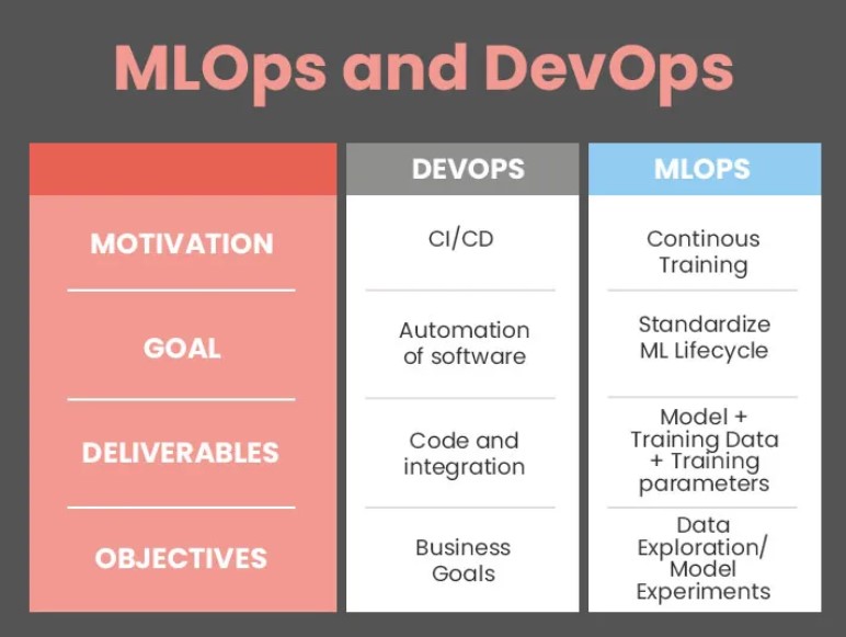
ML model monitoring across many sites, devices and backends rests on three things. Every deployment logs the same telemetry fields, drift checks run on that telemetry beside the serving path rather than inside it, and every alert is broken down by segment before anyone acts on it. The sites do not have to run the same model for you to get one view; they have to log the same things. In an MLOps pipeline, monitoring sits between serving and retraining: it collects inference inputs and outputs, compares them with a baseline on a schedule, emits structured events when thresholds are crossed, and those events trigger retraining jobs, incident tickets or a page to on-call engineers.
One ML model monitoring view across a fleet, without replacing local models
A fleet-wide view comes from a central layer that ingests each site’s inputs, scores and outcomes in one common shape, while each site keeps its own model, stack and release cadence. Uber Engineering’s D3 drift detector shows why the layer has to be automated: it monitors by dimensions such as app version and city on its own, because setting up dimension-based monitors by hand for hundreds of cities was not feasible.
TechnoLynx builds that central layer on top of the telemetry each site already produces, through the Production AI Monitoring Harness. The harness adds the drift jobs and segment-level alerting on top of that telemetry.
Build on what each site logs, or adopt a platform?
None of our sources settles this choice directly, so what follows is our judgement. A Let’s Data Science guide on production MLOps gives the principle we would start from: reuse the infrastructure that already applies and extend its checks to cover how the system actually behaves. Managed platforms are opinionated about where the data lives. Vertex AI Model Monitoring, for example, logs incoming prediction requests to a BigQuery table in your project and analyses those logged features for skew or drift. That suits models already served on Vertex. It does much less for a plant running its own stack on premises.
| Situation across the fleet | Lean towards | Reason |
|---|---|---|
| Sites already log versioned inputs and scores in compatible formats | Build a central layer on existing logs | Aggregation is the only missing piece |
| Schemas differ, but sites share a transport (OpenTelemetry, Prometheus, a message bus) | Build with per-site adapters into one schema | Adapters are cheaper to write than a re-platform |
| Most models already serve on one managed platform | Use that platform’s monitoring and feed its alerts into the central view | Duplicating its drift jobs adds cost without adding signal |
| Sites cannot share raw data | Distributed tests that ship only summary statistics | Local devices compute distances and a central server aggregates them, so raw data never leaves the site |
| No consistent logging anywhere | Instrument first | Any platform you buy would need this instrumentation anyway |
The risk on the build side is pooling everything into one number. When the MMC+ team at Microsoft and Massachusetts General Hospital (2024) monitored the emergency room and an ambulatory operating room separately, the two showed different drift patterns around the same event. A central layer that only reports the pooled number throws that difference away.
What each deployment should log so monitoring data can be split by segment later
A segment you did not log cannot be analysed later. Schema decisions made at ingest decide which root-cause questions you can answer six months on. Microsoft’s Application Insights documentation describes the same pattern for application telemetry: strongly typed context fields such as application version let it correlate behaviour changes with redeployment, and custom properties add dimensions such as the deployment slot that produced the telemetry.
| Field | Why it matters |
|---|---|
| Model version (the immutable version actually loaded, not only the alias) | Moving a registry alias does not restart a serving process (Let’s Data Science), so the version that was loaded has to be recorded per release |
| Site or deployment ID | Lets you monitor each site separately instead of only in a pooled view |
| Device, scanner or camera model, and firmware | CheXstray notes device model and manufacturer metadata can lead to unexpected model results |
| Region | On FMoW, Africa’s class distribution changed faster than the global distribution |
| Backend or provider | gen_ai.provider.name identifies which provider’s telemetry format a span carries |
| Operation type | GenAI conventions separate chat, embeddings, retrieval and other operations by name |
| Trace or operation ID | A root operation ID groups telemetry across multiple components |
| Soft score, not only the thresholded label | Soft predictions carry information about the model’s relative certainty |
| Outcome, joined later through the trace ID | Labels often arrive late, so the join key has to exist from day one |
| Feature pipeline and preprocessing version | Training-serving skew can come from a small change such as different rounding at serving time |
Tracing a flagged drift back to a specific cause
Tracing relies on the trace ID and the version fields above. Application Insights links a request to the dependency calls it triggers through a shared correlation context, so the full flow of an operation can be followed. For a model pipeline, the same correlation lets a drift alert be joined to the upstream event that preceded it, whether that was a feature pipeline release, a new input source at one site or a new firmware rollout. If a pipeline release and a device update land in the same week, the telemetry shows both and cannot pick one for you. The instrumentation side is covered in more depth in our piece on distributed tracing as the foundation of the serving pipeline.
Normalising telemetry from hosted APIs and self-hosted models
A hosted API and a self-hosted model can share one pipeline if both emit spans to the same conventions and carry a provider attribute as the discriminator. The OpenTelemetry GenAI semantic conventions define gen_ai.provider.name for this purpose, with well-known values such as openai, anthropic and aws.bedrock. They also note that the attribute reflects the instrumentation’s best knowledge, which may differ from the real upstream provider when a client goes through a proxy. On the self-hosted side, vLLM exposes end-to-end request latency and inter-token latency histograms on a /metrics endpoint.
A hosted API exposes only what the provider returns. Prompt and response content is also off by default under the OpenTelemetry conventions (NO_CONTENT) and has to be opted into.
On whether one drift metric can serve every model family, the “Failing Loudly” study (Rabanser and colleagues) found that two-sample testing on representations from pre-trained classifiers performed best across the shifts it explored. The FedDrift authors (Jothimurugesan et al., 2023) note that proportional rather than absolute loss thresholds suit setups with several models, because different models have different loss magnitudes.
Running PSI and KS checks more often than monthly without adding serving latency
Drift checks can run hourly or more often without touching scoring latency, provided they read from logged traffic rather than sitting inline in the scoring path. A 2020 paper on monitoring models deployed with KFServing and Seldon Core describes the pattern: a payload logger sends request and response events to a KNative broker, and the outlier and drift detectors consume those events as separate, separately scaled services.
LynxBenchAI publishes measured results for inference accelerators, not for your scoring pipeline, which shows whether the hardware beside the serving path has headroom for more frequent drift jobs; the first step is to look up its results for the accelerators your sites already run.
The checks themselves run fast. In the EAAS reference architecture (2026), per-feature KS and PSI tests ran in under 10 ms for up to ten features and were judged suitable for per-batch monitoring. Approximate MMD took about 500 ms and was suited to periodic evaluation. Walmart’s AIDR anomaly-detection platform, which served predictions from over 3,000 models, runs drift detection as a daily multiprocessing cron job. MLflow’s guidance on drift monitoring puts the cadence anywhere from every few minutes for real-time systems to daily for batch pipelines. Vertex AI’s monitoring jobs run at a minimum granularity of one hour, with a default of 24 hours.
Running PSI on shorter windows has a statistical cost. A 2024 analysis in the Journal of Risk Model Validation shows that PSI’s expected value and variance depend on both the number of bins and the sample sizes. The familiar thresholds (below 0.10 is little change, 0.10 to 0.25 is moderate, above 0.25 calls for action) are used without reference to type I or type II error rates. A PSI of 0.1 therefore means different things at different sample sizes. We would recalibrate thresholds whenever the cadence changes rather than carry them over.
We would keep threshold and feature changes in the model registry, not in a redeploy of the scoring service. MLflow’s aliases name a specific model version (a champion alias, for instance), can be reassigned through the client API, and allow several aliases per version for A/B rollout. Whether a new merchant-category feature or segment-aware rule breaks the latency budget depends on what the feature costs to compute and how slow its data source is, so it has to be measured under load, not assumed. Batching is the other lever. The DNNScaler system, for example, profiles a model and picks the largest batch size that keeps latency within the SLO, adjusting it during production. Two trade-offs remain: asynchronous drift jobs cannot give a true real-time drift alarm, and adding inference capacity for headroom raises inference cost, to weigh against the SLA.
Real degradation or just a different scanner or stain batch?
Drift that remains after controlling for scanner, firmware and site points to a real accuracy drop. Drift that vanishes against each stratum’s own baseline points to benign variation. Scanner differences have a measured effect on performance. A 2024 experimental study across CT, MRI and X-ray datasets found that performance on data from a different scanner was almost always worse than on same-scanner data, with the drop most severe for MRI, moderate for X-ray and small for CT.
The decision rule follows from that. When an alert fires, first check whether the flagged site and scanner fall inside the variation already characterised for that stratum. If they do, treat it as benign and adjust that stratum’s threshold. If drift remains after the known covariates are accounted for, escalate it as model degradation. Per-scanner or per-firmware baselines are worth their cost when variation between strata is large compared with the noise within each stratum; otherwise one global baseline is enough. The MMC+ work shows how a single metadata field can carry the signal: the share of antero-posterior chest X-rays rose from under 20% to over 40% by mid-2020, and AP projection makes the heart look larger, which lowers diagnostic quality for cardiomegaly.
The cross-scanner study tested each model on another manufacturer’s data and repeated every experiment over ten seeds. Three caveats limit this. Rare scanner and site combinations may not have enough history for a reliable baseline. Stress tests only cover the variation you anticipated. The whole decomposition fails if scanner and stain covariates are not logged at inference time.
Which region or firmware mix is behind the accuracy drop?
Root-causing a regression stops being a spreadsheet exercise once every inference event carries model version, region and camera or firmware identifiers. A scheduled job can then rank slices by how much each contributes to the drop. Google’s multi-relational analytics service surfaces that kind of slice view: it powers the Google Analytics Contributor and Trend-Change insights, which highlight interesting slices.
The FMoW benchmark shows why regional effects matter. On the satellite-imagery FMoW benchmark, a model trained on the global dataset reached 48% accuracy on Africa after a major drift in 2014, compared with 66% on the rest of the world, while the global class distribution changed only slowly. An aggregate metric hides that kind of gap.
Read the ranked list like this: if one slice dominates, it is the attributed cause; if the drop is spread across slices, flag it for deeper investigation. Small slices produce unreliable metrics. A firmware rollout that coincides with a seasonal change needs a controlled comparison before you blame either one. If metadata tagging lags behind changes in the field, a stale firmware tag sends the investigation to the wrong place.
Where degradation concentrates: error analysis by subgroup, tested properly
Break the overall metric down by the segments plausibly linked to the risk. Then test each segment, instead of reading point estimates off a dashboard. Error analysis by subgroup is where concentrated degradation becomes visible, and the depth of that method is covered in our article on why one blended metric is not enough for stratified evaluation.
TechnoLynx builds this per-segment breakdown and its tests into the Production AI Monitoring Harness, starting from a segment list agreed before any results are read.
When two model variants are scored on the same items, such as an FP32 model and its INT8 version, McNemar’s test on the paired outcomes is the standard check for whether a per-segment accuracy difference is real. We would treat it as a hypothesis to test segment by segment with a sample size worked out in advance. Strict labelling budgets make this hard. A 2026 study of stratified importance sampling found that combining strata (for example predicted class crossed with model version) with importance weighting gave lower estimator error than either method alone under a fixed labelling budget.
Testing many segments raises the false-positive rate unless you correct for it. The EAAS drift service, for instance, applies Benjamini–Hochberg correction for false discovery rate or Bonferroni for family-wise error across per-feature KS tests. Segment definitions also have to be fixed upfront; segments picked after looking at the results will always turn up a “problem” segment.
How much traffic a region needs before a metric drop means anything
A per-region CTR or watch-time drop is signal only when the region’s sample in the comparison window is large enough to tell that size of drop from noise. That minimum comes from a power calculation for the effect you care about, not from a fixed rule. Each region needs its own sample-size floor and baseline before alerts can be trusted.
TechnoLynx sets up these per-region slices, sample-size floors and baseline periods as part of a Production AI Monitoring Harness build.
EAAS suppresses subgroup metrics below a default of 30 samples to avoid noisy alerts. CheXstray skipped any detection window with fewer than 150 exams. MMC+ went further and attached uncertainty bounds to its drift metric, which keeps small windows from producing spurious drift readings. Those floors suit their own settings and should not be copied across. They show that a floor is part of the design.
How quickly a new region gets a reliable baseline depends on how fast it accumulates traffic, so no single answer applies. Run new and low-volume regions in baseline-collection mode, turn on alerting once the floor is met, and set anomaly sensitivity to the noise that region’s volume implies. Some small markets may never reach a sample size where small drops can be detected within a useful window.
Where model monitoring sits next to the registry, CI/CD and retraining
Monitoring sits between serving and retraining. MLflow describes this wiring: PSI values and prediction drift rates are logged as time-series metrics against a registered model version, alert rules on those metrics connect to retraining workflows, and the registry makes promotion a governed step. The bigger change is moving from fixed-schedule retraining to retraining triggered by drift alerts, so that models are retrained only when the evidence calls for it. MLflow’s registry documentation recommends promoting ML code (training, inference and infrastructure as code) through dev, staging and production via CI/CD, a setup it says extends to model monitoring. This is part of the wider MLOps engineering work of registries, CI/CD and retraining pipelines.
Performance-based drift detection needs feedback on predictions to arrive quickly, and that feedback is not always available. When labels are late, prediction distribution shift is the most reliable early proxy. Label-free estimators also have hard limits: NannyML’s confidence-based performance estimation stays accurate under data drift but does not work under concept drift, which can rarely be identified without ground truth. Our sibling article on monitoring model health without ground truth covers those proxies in depth.
Acting on one site’s monitoring signal without redeploying the fleet
A signal from one site should change that site’s model and nothing else. That only works if the registry is organised the way the fleet is. MLflow suggests registered models per combination of environment and business problem, such as prod.ml_team.revenue_forecasting, with permissions set on each. Adding the site or backend to that combination, with its own alias, lets one plant be rolled back while the other plants keep their versions. Whatever the layout, record the version each site actually loaded and keep the previous release available for rollback. A drift statistic on its own is not a deployment decision: promotion needs representative evaluation, change approval and a tested rollback.
Walmart’s AIDR shows one such loop. The daily drift job identifies the affected models, notifies stakeholders with a preview of the suggested change, and retrains after the customer approves or a timeout passes. After a site-level intervention, the reference baseline has to be re-calibrated too. The MMC+ team re-calibrated their metric with a new reference set from the audited period, which brought it back into its acceptable range. Setting those per-site thresholds and triggers has its own trade-offs, which we cover in designing segment-aware drift monitoring and retraining triggers. Each fleet still has to decide who owns the decision once a site’s alert fires. MLflow’s guidance notes that leaving that question open until a model fails is a governance gap that keeps showing up in post-mortems.
Who can build fleet-wide model monitoring across our sites and backends?
TechnoLynx builds monitoring that spans mixed estates of plants, regions, hosted APIs and self-hosted GPU models, on top of the logging each site already has. On build versus specialist: an in-house team with spare MLOps capacity and consistent logging can extend its own stack. A specialist earns their place when the schemas differ, the backends are mixed and the segment analysis needs statistical care. When choosing a partner, ask how they handle per-segment sample sizes and multiple testing, and whether they leave your models in place. The engagement is the Production AI Monitoring Harness, and Production AI Reliability covers running the monitoring once it is live.
This engagement does not suit a fleet that already serves everything on one managed platform; that platform’s built-in monitoring is the simpler route. We would point teams that mainly want LLM trace dashboards to an observability product. In clinical or credit settings we deliver the engineering, while regulatory sign-off stays with your validation and compliance owners.
FAQ
How do you identify data drift?
Compare each feature’s current distribution with its training baseline: PSI for binned comparisons, the Kolmogorov–Smirnov test for continuous features, and chi-squared tests for categorical ones.