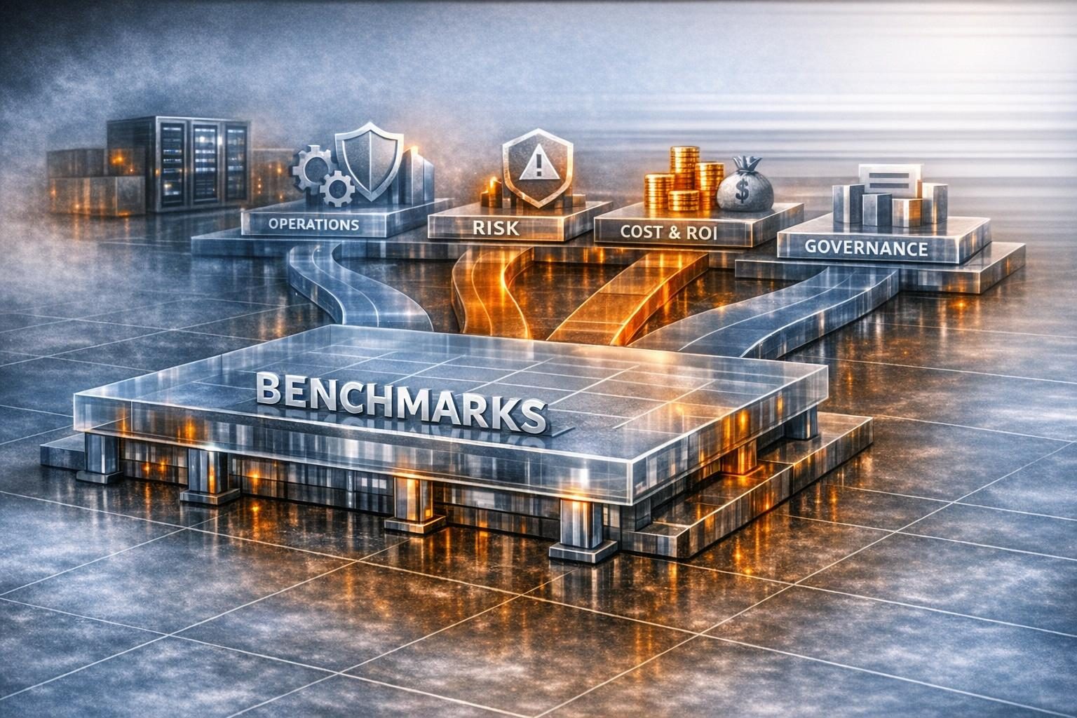
Two Different Multi-GPU Questions: Planning vs Validation

Planning GPU capacity for a new workload and validating a multi-GPU deployment you already run are two different questions, and they need different tools. Planning looks forward. Given an arrival rate and a latency SLO, it asks how many GPUs you need, what batching and queueing design to use, and what should trigger autoscaling. Validation looks backward. It asks whether the GPU cluster you already have reaches the throughput its node count should give, and whether it still produces correct results. Planning is arithmetic over batch size, latency and queueing. Validation is profiling, comparison against published scaling results, and known-answer checks.

TechnoLynx handles both through GPU Performance Engineering, and the first step is the same for either: an end-to-end profile of the inference pipeline with its latency broken down stage by stage, so the sizing assumptions or the shortfall rest on measured numbers.

Mixing the two up is costly in both directions. If you validate a planned cluster on average utilisation alone, you miss tail-latency failures. If you plan a new cluster by extrapolating from a run nobody has profiled, you build its hidden bottleneck into the purchase order.

Planning versus validation at a glance

	Capacity planning (new workload)	Validation (existing deployment)
Direction	Forward: what to provision for a target rate and SLO	Backward: whether what you run delivers what it should
Core inputs	Arrival rate, latency SLO, measured batch-latency profile per model	Profiler traces, log counters, collective bandwidth, reference results
Main method	Largest batch that fits the SLO, then GPUs = rate / per-GPU throughput	Profile the critical regions and compare scaling efficiency with published runs
Checked with	Queueing simulation of real arrival traces	Known-answer and conservation checks for correctness
Typical failure caught	A fleet at low average utilisation that still breaks its P99 SLO	A run that scales badly through load imbalance, or runs fast but gives wrong answers

Sizing a GPU cluster for a new throughput target

Worked example: from a latency SLO to a GPU count

The Nexus paper (SOSP 2019) gives a simple sizing rule. Use the largest batch size that still meets the latency SLO, and keep the batch execution cost at no more than half of that SLO. The reason for the half is mechanical: a request that just misses a batch waits for the next one, so its worst-case latency is twice the batch execution cost. In the paper’s example, a 200 ms SLO allows a maximum batch of 16, which gives 160 requests per second per GPU, so the GPU count is the observed request rate divided by 160.

To apply this to a new line speed, the working runs in four steps:

Measure batched latency for your model at several batch sizes. Nexus found a linear fit, latency = αb + β, often adequate, where β is the fixed invocation cost and α the cost per extra item.
Find the largest batch B whose latency is at most half the SLO, and take per-GPU throughput as B divided by that latency.
Take the total arrival rate: with N cells each sending f frames per second, the fleet sees N × f requests per second, assuming every frame is a request.
Divide the arrival rate by the per-GPU throughput. The result is a floor, not a plan.

That floor is optimistic by construction. Nexus’s own lower bound assumed full batchability, the optimal batch size and back-to-back scheduling. On that basis the paper computed a bound of 9.8 GPUs, while Nexus actually used 11.7, about 84% of the theoretical efficiency.

Three things push the real requirement further above the floor. Non-DNN work such as preprocessing can take up to 56% of a request’s time on a medium-sized image even in an optimised server, according to a 2024 study of DNN server overheads. Nexus also needed 4 to 5 CPU cores to saturate one GPU. And queueing matters more than averages suggest: a 2026 fleet-planning study found that a fleet at roughly 30% utilisation measured a P99 time-to-first-token of 1,052 ms, because long-tail service events caused cascading back-pressure. Its analytical model approved fleets that a discrete-event simulation then showed to be broken.

The practical implication is that your headroom figure should come from replaying a realistic arrival trace, not from a utilisation target. For pipelines with several models (detect, then recognise), the end-to-end SLO also has to be split between stages. Nexus gave 345 ms of a 400 ms budget to detection, and splitting the budget evenly instead cost 19% of throughput. The wider pre-purchase questions about topology, networking and scheduling are covered in sizing and proving out a multi-GPU cluster before you buy.

Should you use Triton dynamic batching or a custom scheduler, and what latency does each add?

In the benchmark below, NVIDIA Triton’s dynamic batcher raised throughput at a small, tunable latency cost. A 2026 healthcare inference benchmark on Kubernetes measured Triton at 420 req/s without batching and 780 req/s with dynamic batching at batch size 16. Over the same change, median latency rose from 28 ms to 34 ms and p95 from 52 ms to 60 ms.

The setting that controls this trade-off is max_queue_delay_microseconds. When a full or preferred-size batch cannot be formed, it caps how long a request may wait for others to join, and the batcher sends whatever it has once that delay expires. With default settings Triton builds the largest batch it can and adds no delay. NVIDIA’s documented procedure is to measure the default with Performance Analyzer and then raise the maximum batch size or the delay until the latency budget is exceeded. NVIDIA also states that the benefit of dynamic batching and multiple model instances is model-specific. Two instances per model often help because memory transfer overlaps with compute.

The delay trick works outside Triton too. In Clipper (NSDI 2017), a 2 ms batch delay gave a 3.3x throughput gain on a model with a high fixed cost per batch.

A custom scheduler earns its cost in a few specific cases:

several models share GPUs under different SLOs;
you need admission control that drops requests early rather than letting batches shrink;
the SLO has to be split across a multi-model query.

Nexus’s early-drop policy reached up to 25% higher throughput than lazy dropping in simulation. Clockwork (OSDI 2020) rests on DNN inference having predictable execution time on a GPU. That predictability breaks once batches run concurrently: a 2025 study on an L4 measured interference of up to 151.66% at the 95th percentile with only two concurrent batches. Any custom scheduler that packs work aggressively has to model that interference or accept missed deadlines.

What should trigger autoscaling when a cell’s frame rate spikes?

Scale on queue depth, with GPU activity as a secondary signal, and never on CPU utilisation alone. The authors of the Triton-on-Kubernetes benchmark scaled on 60% CPU utilisation. They call it a lagging indicator for GPU workloads and propose DCGM-based GPU-aware autoscaling as future work.

Triton exposes the signals directly. Pending request count is effectively the per-model queue size, nv_inference_queue_duration_us accumulates time spent in the scheduling queue, and GPU utilisation comes through DCGM. Cast AI points to DCGM_FI_PROF_GR_ENGINE_ACTIVE as a proxy for inference saturation and calls request queue depth the more accurate scaling signal.

How fast scaling reacts limits what autoscaling can absorb. Cast AI puts a full cold start, from node provisioning to model load, at typically 8 to 15 minutes for large models. Kubernetes HPA adds its own damping on top: a tolerance band below which it will not scale, stabilisation windows, and a default 30-second initial readiness delay. Even Nexus, re-planning in 30-second epochs, took 12 seconds to detect a demand change, and dropped requests in the meantime.

A spike shorter than your scale-up path has to be covered by provisioned headroom or warm replicas, not by the autoscaler. Cast AI advises keeping at least one warm pod for latency-sensitive serving.

Validating an existing multi-GPU deployment’s throughput

The two halves meet in one measured number. Clipper gained 3.95x throughput on four GPU replicas, from 19,500 to 77,000 qps, because GPU inference was the bottleneck and the RPC layer could keep the GPUs saturated. A planner would happily assume near-linear scaling from that result. A validator has to confirm that the same conditions hold in their own deployment. A 2024 study shows a case where they break: for large images, where preprocessing was the bottleneck, adding GPUs beyond two gave only marginal gains.

How do you profile a multi-GPU run to confirm it reaches the expected throughput for its node count?

Start from the counters the software already writes, then narrow down with a profiler. For GROMACS, the end of md.log reports cycle counters, wall time per part of the step, and the PP/PME load ratio, with a warning when imbalance costs a lot of performance. Matom·steps/s is timestep-independent and normalised by system size, giving a measure of simulation efficiency.

Time listed as “Wait GPU NB local” means the CPU is waiting for non-bonded work on the GPU. Launch overhead of a few percent is normal, but multi-GPU runs can show 10% or more.

For Nsight Systems, limit the capture to performance-critical regions with cudaProfilerStart()/cudaProfilerStop() or NVTX ranges, and leave the test harness’s initialisation and correctness checks outside the profile. For inference servers, Triton’s split of queue time from compute time shows whether the shortfall comes from scheduling or from the GPU. Average batch size can be derived from the count metrics.

Interconnect performance needs one correction before you compare it with a spec sheet. nccl-tests reports algorithm bandwidth (size over time), and that number falls as the rank count rises. Bus bandwidth applies a factor per collective, 2(n−1)/n for AllReduce, so that it can be compared with the hardware peak. At 8 ranks the AllReduce factor is 2 × 7/8 = 1.75, so bus bandwidth is 1.75 times algorithm bandwidth.

In a 2026 GROMACS–DeePMD study, profiling showed collective time to be negligible next to inference. The dominant penalty was synchronisation caused by load imbalance. A broader treatment of profiling-based validation for GPU workloads and cross-model benchmarks covers the method beyond multi-GPU runs.

Is your CPU-to-multi-GPU speed-up in line with published GROMACS and RELION scaling?

Compute your scaling efficiency first: speed-up divided by GPU count. Then compare it only against published runs of a similar system size, because scaling depends strongly on size. Useful reference points:

GROMACS with a deep-potential model, 15,668 atoms (2026): strong-scaling efficiency of 66% at 16 devices and 40% at 32, on A100 and MI250X.
GROMACS heterogeneous parallelisation (2020): good relative scaling up to 8 GPUs (50% efficiency), after which the single PME GPU became the bottleneck.
GROMACS 2023 with PME GPU decomposition (NVIDIA): the 12-million-atom benchPEP-h benchmark ran 21x faster than the legacy code path on 64 nodes (256 A100 GPUs).
Classical MD on CPU nodes (2025): a 20k-atom system scaled poorly, a 61k-atom system scaled well to about 8 nodes, and larger systems scaled linearly to 16.
RELION-2 (2016): classification and high-resolution refinement accelerated by more than an order of magnitude, and a quad-GPU workstation outperformed a large cluster job in 3D classification.

If your run is below these, look for performance left on the table. Too many MPI ranks per GPU is a known inefficiency, with 1 to 3 generally optimal and 1 rank per GPU usually best in GPU-resident mode. Near the scaling limit of about 10,000 atoms per GPU, communication latency dominates. Larger nstlist values (200 to 300) often beat the conservative automatic setting in multi-GPU runs.

If your run is above them, ask whether you are comparing like with like. The 2025 biomolecular platform study notes that most MD jobs still run best on single GPUs, and that domain decomposition scales favourably only for very large (>10M atom) systems. It also found that scaling to many nodes can triple the energy used per nanosecond simulated. The MPI-NAT benchmark set spans 6k to 12M atoms.

What sanity check catches a multi-GPU result that is fast but wrong?

Run a calculation whose answer you know before you trust a calculation whose answer you don’t.

Known-answer reduction. A 2026 five-GPU statistics study first summed an index column running from 1 to 10 billion. Because the analytical sum was known, any discrepancy pointed straight to parsing, partitioning or reduction logic. For an index from 1 to n the expected sum is n(n+1)/2.
Precision at scale. The same study warns that at very large N, catastrophic cancellation can make mathematically correct workflows produce unstable results. It cites covariance terms formed independently and then subtracted as the example.
Physical invariants. In MD, a run that does not conserve total energy means the integrator is unstable for that hardware and software combination. The 2025 study saw random energy spikes in a 1,400k-atom GROMACS run on MI250X. Energy conservation is a coarse check, and passing it does not rule out numerical problems.
Reference agreement within run-to-run noise. RELION-2 single-precision GPU refinement reached a gold-standard FSC indistinguishable from double-precision CPU refinement. Its angle assignments differed by about as much as two CPU runs with different random seeds. Compare GPU against CPU on the same footing, with seed-to-seed spread as the tolerance.
Stability of a structural observable. The GROMACS–DeePMD work tracked radii of gyration. A sustained increase would have signalled an error in the model or the domain decomposition.

The 2026 statistics study put correctness and infrastructure checks before any performance tuning. Of the habits in this article, that one is the most worth copying.

Who can size a new GPU cluster or check the one we already run?

TechnoLynx profiles multi-GPU inference pipelines end to end through GPU Performance Engineering, for a new throughput target or a deployment that falls short. Both start with end-to-end profiling of the pipeline and a stage-by-stage breakdown of its latency. For planning, that profile supplies the per-GPU throughput and the preprocessing and queueing costs that the batch and GPU-count arithmetic depends on. For validation, its stage-by-stage breakdown shows where time is lost, so that the fix targets the right layer. Where the open question is which accelerator to buy, LynxBenchAI is the measuring tool: it benchmarks accelerators on one scale. It does not run your own workload, so your model’s batch-latency profile still has to be measured.

This work does not suit every team. Buyers looking only for extra hours, or for the cheapest hardware quote, are better served by their cloud provider’s or hardware vendor’s sizing support. For scientific codes, TechnoLynx takes on the engineering part: throughput and scaling. Whether a force field or reconstruction is scientifically valid stays with the domain scientists.

Why the validation result feeds the next plan

A capacity plan divides an arrival rate by a per-GPU throughput, and that throughput is itself a validation result. If it comes from a vendor datasheet or an unprofiled run, every GPU in the plan carries the same error. The next step we would take is to measure how bursty traffic is per cell at the new line speed, and how long spikes last compared with your scale-up time, then replay that trace before fixing headroom.