AI in computer vision means that learned models replace hand-crafted features: instead of engineers designing features for each problem, deep networks learn problem-specific features automatically. A vision system does not “see” the way human vision does. It samples numbers off a sensor and passes them through layered transformations until something useful comes out. AI’s contribution is learning those transformations from data instead of relying on hand-crafted features. This article stays with the engineering: how a frame becomes a decision, which models do the work, and what that looks like on a factory line or inside a vehicle.
A quick note on terms, since people often ask about computer vision vs machine learning. Computer vision is the problem: getting meaning out of images and video. Machine learning is a family of methods, and modern vision systems use it heavily, but a vision system can also be built from classical geometry and image processing with no learning at all. Today almost every neural network used in computer vision is deep and relies heavily on convolution layers.
How AI in computer vision turns a camera frame into a decision
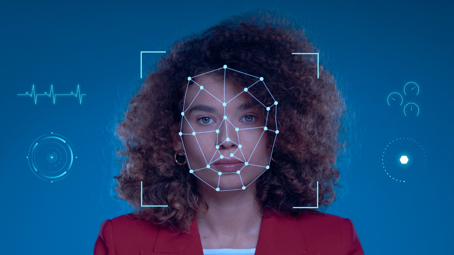
Computer vision is useful in production because a four-stage pipeline (detection, alignment, embedding, matching) turns pixels into decisions a system can act on. The question worth asking is not whether the AI “looks at images” but which stage of that pipeline owns which failure mode. If you know that, you can tell a lighting problem from a model problem from a database problem.
| Stage | What it does | Where we would expect it to fail |
|---|---|---|
| Detection | Finds candidate objects or regions in the frame | Missed objects as scenes get more crowded |
| Alignment | Normalises each region (crop, rotate, rescale, register to a template) | Any error here passes to every later stage |
| Embedding | Turns the aligned region into a feature vector or class score | Fails when lighting or optics change between training and production |
| Matching | Compares the embedding against references, thresholds or rules to produce a decision | A threshold tuned on one data distribution and applied to another |
In a modular, observable pipeline, when a decision goes wrong you can find the stage that produced the bad intermediate. For a slower walk through the sensor-to-output chain, see our article on how computer vision works step by step. Video adds a time dimension, which is where recurrent networks for video and other sequence models come in.
Classification, detection and the two kinds of segmentation
The first stage can produce very different kinds of output, and choosing the wrong one over-builds or under-builds the system. The four standard tasks differ in what they label:
| Task | Output | What it cannot tell you |
|---|---|---|
| Classification | One or more labels for the whole image, such as “dog” or a specific breed | Where the object is, or how many there are |
| Object detection | A box and a class label for each object; training needs every object hand-annotated with a rectangle and label | The object’s exact outline |
| Semantic segmentation | A class label for every pixel (road, sky, person, car) | Which pixels belong to which individual car; all cars share the label “car” |
| Instance segmentation | A class label plus a separate mask for each object instance | Nothing extra is free: it is generally harder, since it has to classify correctly and also separate overlapping objects |
Panoptic segmentation combines the two segmentation forms. In practice the split matters: a robot arm picking one part out of a bin of identical parts needs instance segmentation, while marking where a vehicle can drive is a semantic segmentation problem.
Which model families do the work
Convolutional neural networks (CNNs) gained popularity because they learn features and patterns straight from raw images. Their filters respond to local patterns, and pooling layers reduce dimensionality and add robustness to variation. Residual learning eased the training of much deeper networks, up to 152 layers, and an ensemble of these residual nets reached 3.57% error on the ImageNet test set (He et al., 2015). YOLO (Redmon et al., 2015) treated detection as one network regressing boxes and class probabilities from the full image in a single pass, and ran at 45 frames per second, with a smaller variant at 155.
Vision Transformers (ViTs) drop convolution altogether. Dosovitskiy et al. (2021) showed that a pure transformer applied to sequences of image patches does very well on image classification when pre-trained on large amounts of data. Self-attention lets a ViT model long-range relationships across the whole image instead of a local receptive field. That advantage has a cost. ViTs assume little prior knowledge about images, so they depend heavily on large datasets, they can underperform CNNs when training data is small, and their attention mechanism is expensive in computation and memory.
Hybrid CNN-Transformer models use convolutional layers to capture local features and then pass them to transformer layers for global context. One way to see the two pure families:
| Family | Good at | Weak where |
|---|---|---|
| CNN (ResNet, YOLO-style detectors) | Local patterns, small datasets, less compute than ViTs | Larger, complex patterns spread across the image |
| ViT | Global relationships, large pre-training corpora | Small data and tight compute budgets |
No single architecture is best everywhere. The dissertation Exploring the Design Space of Deep Convolutional Neural Networks at Large Scale reports that, to the author’s knowledge, no single CNN solves all problems optimally, and the right architecture depends on the application.
Classic machine vision versus deep learning: where each still wins
Classical machine vision depended on hand-crafted features, and deep learning replaced that with problem-specific features learned automatically. The swap is not a one-way upgrade. A 2022 segmentation survey (Minaee et al.) reports broad agreement that deep segmentation performance is plateauing in some domains and argues for combining CNNs with classical model-based methods such as active contours and graph cuts.
We would keep classical methods where the geometry is fixed, the lighting is controlled and the result has to be a traceable measurement (a gap width, a hole position, a barcode). Rules are easier to verify there. Deep learning earns its place when defect appearance varies too much to write down, as with cracks, scratches, contamination and cosmetic flaws on textured surfaces. We would build inspection systems from both: classical alignment and measurement, and a learned model for the judgement call.
Real examples on factory lines
Quality control is where computer vision is particularly useful in manufacturing. Models trained on camera images can find surface blemishes, dimensional inaccuracies and assembly errors, and they inspect continuously.
BMW Group has described its own production use. AI compares component images in milliseconds with hundreds of other images from the same sequence, to check whether every required part is fitted and in the right place. At the Dingolfing final inspection, the system compares vehicle order data with a live image of the model designation and alerts the team when they do not match. BMW says its earlier camera systems sometimes flagged pseudo-defects, meaning deviations that were not real faults, and that these stopped once the network could draw on roughly 100 real images per feature: 100 of the perfect part, 100 with dust, 100 with oil droplets, and so on. These are BMW Group’s own descriptions of its own plants.
Published research gives a measured view of the same idea. Tabernik et al. (2019) built the Kolektor Surface-Defect Dataset from a real quality-control case: 399 images of electrical commutators, only 52 of them showing a defect. Their segmentation-based network reached 99.9% average precision with zero false positives and one false negative. To catch every defect it needed only 3 of the 399 images sent for manual inspection, a 0.75% inspection rate. At that same zero-miss setting, standard DeepLabv3+ and U-Net networks needed 68 and 108 manual verifications. Performance stayed above 99% average precision with 25 defective training samples and fell to around 96% with 5.
The data caveats in that work are just as instructive as the results. Defects were scarce: the dataset reflects a real case where few defective items were available for training. The authors also say their approach is limited to problems that can be framed as pixel-wise segmentation, and that tasks like finding missing parts on complex 3D objects call for detection methods instead. Lighting is the third trap. Cognex’s VisionPro Deep Learning documentation warns that lighting and optics must stay consistent between training and production, because a tool trained under one setup will fail if that setup changes on the line. Variation you expect, such as brighter or darker frames, has to be in the training set. More on industrial use is in our piece on computer vision for manufacturing.
Edge latency follows architecture and memory bandwidth, not TOPS
Practical deployment often requires running models on embedded devices, where low latency, limited memory bandwidth and tight energy budgets dominate. High accuracy is necessary, but deployable applications also depend on inference speed and whole-system energy efficiency. Energy per frame is a single metric that captures these efficiency goals. At 15 frames per second on a 30 W budget, the system has 2 joules per frame (30 W × 1/15 s).
A benchmark of nine YOLO variants on three Rockchip SoCs shows that real performance depends on more than nominal TOPS ratings. On the entry-level RV1106, Nano models needed 68–97 ms and Medium models more than 250 ms. On the RK3588 in single-core NPU mode, Nano models ran in 21–30 ms, fast enough for 30 FPS. Latency tracked detection accuracy (mAP) more closely than parameter count or FLOPs. YOLO11n has fewer parameters than YOLOv8n and was slower on all three chips, which the authors attribute to newer modules adding overhead that maps poorly onto the NPUs. Moving from 0.5 to 1 to 2 TOPS improved latency less than proportionally, and three-core scheduling on the RK3588 gave marginal or even negative gains. Memory pressure hurt more: on the RK3568, YOLOv5n latency rose by more than 270% under heavy memory load, while CPU load slowed it far less. The authors conclude that FLOPs alone do not predict real inference cost, and that models should be benchmarked on the target SoC.
An evaluation of YOLOv8, EfficientDet Lite and SSD across Raspberry Pi and NVIDIA Jetson devices points the same way. On a CPU-only Raspberry Pi 3, SSD v1 took 427 ms and YOLOv8 models took 2,548 to 12,960 ms. Adding a TPU brought SSD v1 down to 61 ms. The accelerator also changed accuracy. YOLOv8 lost accuracy on the TPU-equipped Pis because that deployment required conversion to TFLite and a 320×320 input, so a model name alone tells you little without its format, resolution and quantisation path. Scene content mattered too: lightweight and heavy models scored similarly on simple scenes, and the gap widened as object count grew. Most segmentation models are still far from camera frame rates. The Minaee survey notes that FCN-8 takes roughly 100 ms on a low-resolution image, against the 25 frames per second that camera-rate applications such as autonomous vehicles need.
What we take from this: decide the model and the device together, test them on scenes as cluttered as the real ones, and treat TOPS on a datasheet as an upper bound, not a forecast. LynxBenchAI benchmarks accelerators to inform this choice.
How do vision systems go from recognising objects to acting on a scene?
Recent systems move past recognition by dropping the fixed label set and by connecting perception directly to action.
The first limit is the fixed label set. Standard vision models predict a predetermined set of categories, and every new concept needs more labelled data. CLIP (Radford et al., 2021) trained an image encoder and a text encoder together on 400 million image-text pairs, so natural-language class names can serve as a classifier with no task-specific training. Zero-shot, it matched the original ResNet-50 on ImageNet at 76.2% without using any of the 1.28 million training examples. It was also weak on specialised tasks, including German traffic-sign recognition and estimating distance to the nearest car. Both are self-driving tasks.
Action is the second step. RT-2 (Brohan et al., 2023) encodes robot actions as text tokens inside a vision-language model, so a single end-to-end model maps observations to actions. In 6,000 evaluation trials it handled commands absent from the robot training data and simple reasoning, such as picking the smallest object. Waymo’s EMMA (Hwang et al., 2024) builds on a multimodal language model and maps raw camera data directly to planner trajectories, perception objects and road-graph elements.
What the Tempe crash says about modular perception
The NTSB’s report on the 2018 Tempe crash shows what a perception system logged before it acted. The automated driving system first detected the pedestrian 5.6 seconds before impact, classified her first as a vehicle, then alternated several times between vehicle, bicycle and other. The design discarded tracking history for objects whose classification changed, and it did not account for pedestrians crossing outside a crosswalk. It recognised an imminent collision only 1.2 seconds before impact. The NTSB’s investigation focused on safety culture and risk management. The logged data show that tracking held while classification oscillated and tracking history was discarded.
The system’s data recorded detection time, classification and predicted paths. That is why TechnoLynx defaults to modular, transparent, observable vision systems over end-to-end magic: when something breaks, you need to know where and why. The defect-detection study above also split the work into stages. Tabernik et al. trained the segmentation network first, froze it, then trained a separate decision network, and credit their lead to that two-stage design plus a larger receptive field. For tools that inspect what each model has learned, see visual analytics of what networks learn.
When a team needs a pipeline like this designed, made observable, or moved onto edge hardware, that is the work of TechnoLynx’s computer vision R&D practice.
The decision that remains open
The question we would put to a team is no longer whether AI can recognise the objects. It is where they can accept a decision whose cause they cannot trace to a stage. A foundation model that maps pixels straight to a trajectory may generalise better than a hand-built pipeline, yet when it fails, the log shows only one wrong output. A modular pipeline gives you four places to look, at the price of more integration work. Before choosing a model family or a chip, settle which intermediate results you will need to inspect after a failure, and build so that they exist.