A deep learning recommendation model is not just another neural network you train once and forget. The behaviour of a DLRM is dominated by its sparse embedding tables — the part that learns a vector for every user, item, and campaign — and those tables go stale faster than any other component you deploy. Treat a DLRM the way you treat an image classifier — train the checkpoint, ship it, watch the accuracy dashboard — and you will miss the failure that actually costs you money: silent recommendation decay.
That distinction is the whole point of this article. A DLRM’s parameters are split unevenly between two very different kinds of layers, and the fragile half is the half that most monitoring never looks at.
How does DLRM actually work?
Meta’s published DLRM architecture—the same one MLPerf adopted for its recommendation benchmark—consists of three distinct components. Dense (continuous) features go through a bottom multilayer perceptron. Sparse (categorical) features — user ID, item ID, campaign, category, device — go through embedding tables, one lookup per feature, each returning a learned vector. Those vectors are then combined pairwise in a feature-interaction layer (typically a dot-product), and the result plus the dense output feeds a top MLP that emits a click or conversion probability.
The uneven split matters. The dense MLPs are small — a few million parameters, the same order as a modest vision backbone. The embedding tables are enormous, because they carry one row per categorical value. A catalogue with tens of millions of items and hundreds of millions of users produces embedding tables measured in tens or hundreds of gigabytes, dwarfing the dense layers by two or three orders of magnitude. Most of the model, by memory, is a giant lookup table of learned identity vectors.
In practice this means a DLRM is memory-bound, not compute-bound. The dot-product interaction is cheap; the expensive operation is fetching the right rows out of a table too large to fit comfortably on one accelerator. That single fact drives almost every production decision that follows — where the model lives, how you shard it, and, crucially, how it decays.
Why the sparse embedding tables matter more than the dense layers
Shipping a production DLRM teaches you something training alone never reveals. The dense layers learn how features interact — the general shape of what makes a recommendation good. That shape is relatively stable. The embedding tables learn what each specific entity means right now — and “right now” moves constantly.
Every new user starts with an untrained (effectively random) embedding. Every new item in the catalogue starts the same way. When a campaign launches, the campaign feature’s embedding is cold. When user behaviour shifts — a season changes, a trend spikes, a product goes viral — the meaning of existing embeddings drifts even though the table hasn’t changed. The dense weights can be months old and still be fine. The embedding tables can be a week old and already be lying to you.
This is why the categorical side dominates DLRM’s real-world behaviour. A stale embedding table produces recommendations that are internally consistent and plausible — the model is confident — but wrong, because the vectors describe a catalogue and an audience that no longer exist. Nothing about the model’s own outputs flags this. The loss on the training distribution looks fine. The problem lives entirely in the gap between the table’s frozen view and the world’s current state.
Why does a DLRM decay silently in production?
Accuracy monitors miss silent decay entirely, yet it represents the most insidious failure mode in recommendation systems.
A classifier that breaks tends to break loudly: confidence collapses, an out-of-distribution monitor fires, an obviously wrong label reaches a human. A DLRM does none of that. It keeps returning ranked lists with sensible-looking scores. Click-through and conversion lift erode gradually — in engagements and public post-mortems we’ve seen this land in the range of 10–20% relative decline before anyone attributes it to the model (observed pattern across recommendation deployments; not a benchmarked rate, and highly catalogue-dependent). By the time someone says “the model got worse,” weeks have passed and the causal chain back to a catalogue shift is cold.
The reason it stays silent is that the signal you need is not in the model’s outputs — it is in the inputs. What catches DLRM decay is drift monitoring on the categorical feature distributions themselves:
- Coverage drift — the fraction of requests hitting embeddings that were cold or under-trained at the last training cut. A rising cold-start rate means the catalogue has moved under the table.
- Distribution drift — population shift in which items, categories, and campaigns actually appear in traffic, compared with the training snapshot.
- Freshness lag — wall-clock age of the newest catalogue and interaction data reflected in the deployed embeddings.
- Outcome drift — realised click-through and conversion against predicted, sliced by cohort, so decay shows up per-segment before it shows up in the aggregate.
These are input- and outcome-space signals, not accuracy metrics on a frozen test set. If you want the broader framing of what to instrument once a model is live, our guide to the performance metrics worth tracking in production covers the monitoring layer a DLRM plugs into. Drift on the sparse features is the DLRM-specific addition on top of that baseline. Building that monitoring layer is core to the MLOps engagement pack we run for recommendation and ranking systems.
What an MLOps pipeline for DLRM needs that a static model does not
Retraining cadence determines whether your engagement metrics rise or fall over time. A static model deploys a checkpoint. A DLRM needs a loop wired around it. The table below contrasts the two.
DLRM pipeline requirements vs. a static model
| Concern | Static model | DLRM pipeline |
|---|---|---|
| Retraining | Manual, event-driven | Automated, triggered by drift + on a fixed cadence floor |
| Trigger signal | Accuracy drop on holdout | Coverage/distribution drift on categorical features |
| Versioning unit | Model checkpoint | Checkpoint plus embedding-table snapshot |
| Cold start | Ignored | Explicit init policy for new users/items/campaigns |
| Rollback | Redeploy prior checkpoint | Roll back checkpoint and matching embedding version together |
| Time-to-recover | Weeks (manual diagnosis) | Hours (pipeline re-fits and redeploys) |
Three of those rows are DLRM-specific and worth dwelling on. Embedding versioning matters because a checkpoint and its embedding tables are not independent — a rolled-back top MLP paired with a newer embedding snapshot will produce garbage, so the two must version and roll back as a unit. Retraining triggers must fire on input drift rather than output accuracy, because output accuracy is exactly the thing that stays deceptively healthy. And a cadence floor matters because some drift — slow audience shift — never trips a threshold but still accumulates; a scheduled retrain catches what the trigger misses.
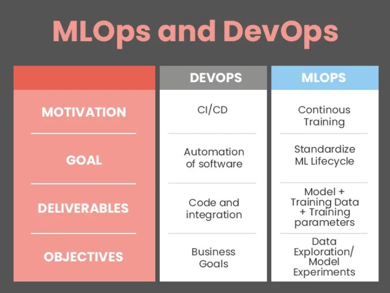
Teams that wire this correctly recover relevance in hours after a catalogue shift rather than the weeks it takes to diagnose decay by hand. That recovery time is the ROI: the recurring cost of skipping the loop is revenue leaking out with no alert attached to it. This is one concrete instance of the general argument that MLOps adds retraining, versioning, and rollback stages a plain deployment lacks — we lay out that full lifecycle in the stages MLOps adds to a DevOps pipeline. DLRM is a stress test for those stages precisely because its fragile part is invisible to naive monitoring, and it is exactly the kind of case MLOps as the operating model that keeps production ML healthy has in mind when it treats retraining and rollback as platform-level, not model-specific, disciplines.
How do you size compute for a DLRM given its embedding tables?
Memory capacity and bandwidth constrain DLRM sizing far more than compute throughput does.
For training, the embedding tables are the constraint. When the tables exceed a single accelerator’s HBM, you shard them — model-parallel embeddings across devices, data-parallel dense layers — which turns the interconnect into the bottleneck. This is why DLRM training benefits disproportionately from NVLink and high-bandwidth all-to-all collectives (NCCL) to move the sharded lookups: the dense compute is trivial next to the cost of gathering embedding rows across the fabric. Frameworks like NVIDIA Merlin / HugeCTR and PyTorch’s TorchRec exist specifically to manage sharded embedding tables and the resulting communication pattern.
For serving, the question is whether the tables live in GPU HBM, in host RAM, or in a dedicated parameter server. Small tables fit in HBM and serve fastest. Large tables often live in host memory or across a distributed store, and the serving latency budget then depends on the lookup and transfer path, not the arithmetic. Provisioning this well is a hardware-topology decision — HBM capacity, PCIe versus NVLink transfer paths, and how the table shards map onto that topology — which is why teams sizing infrastructure for DLRM retraining and serving move into GPU provisioning and performance engineering as the next question. The two problems are joined at the hip: how you shard the embeddings dictates the interconnect you need.
FAQ
How should you think about dlrm in practice?
Deep Learning Recommendation Models split input features into two parallel processing paths: continuous signals pass through a bottom multilayer perceptron while categorical identifiers retrieve learned vectors from sparse embedding tables before merging in a feature-interaction layer that feeds a final MLP predicting engagement probability. In practice the embedding tables hold almost all the parameters, so the model is memory-bound rather than compute-bound — which shapes every downstream decision about serving, sharding, and monitoring.
What makes DLRM different from a standard deep learning model — why do the sparse embedding tables matter more than the dense layers?
The dense layers learn how features interact in general and stay relatively stable; the embedding tables learn what each specific user, item, and campaign means right now, and that meaning shifts constantly as the catalogue and audience move. The tables also dominate by memory, often by two or three orders of magnitude. So the fragile, fast-decaying part of a DLRM is the categorical side, not the dense side.
Why does a DLRM decay silently in production, and what kind of drift monitoring catches it?
A DLRM keeps returning plausible, confident-looking recommendations even when its embeddings describe a catalogue that no longer exists, so accuracy dashboards on a frozen test set never fire. The signal lives in the inputs and outcomes: coverage drift (cold-embedding hit rate), distribution drift on categorical features, embedding freshness lag, and per-cohort outcome drift. Watching those input- and outcome-space signals catches decay that output accuracy hides.
What does an MLOps pipeline for DLRM need — retraining triggers, embedding versioning, rollback — that a static model does not?
It needs automated retraining triggered by input drift (not by output accuracy, which stays deceptively healthy), plus a cadence floor to catch slow drift that never trips a threshold. It needs embedding-table versioning so the checkpoint and its embeddings roll forward and back as a single unit, and an explicit cold-start policy for new entities. That loop turns weeks of manual “the model got worse” diagnosis into hours of automated recovery.
How do you size compute for training and serving a DLRM given its large embedding tables?
Size for memory capacity and bandwidth first, since the tables dwarf the dense compute. Training large tables means sharding embeddings across devices, which makes the interconnect (NVLink, NCCL all-to-all) the bottleneck. Serving depends on where the tables live — GPU HBM for small tables, host RAM or a distributed parameter store for large ones — so the latency budget is dominated by the lookup and transfer path rather than the arithmetic.
When is DLRM the right choice for a recommendation problem, and when is a simpler model enough?
DLRM earns its complexity when you have high-cardinality categorical features, a large and shifting catalogue, and enough interaction data to keep the embeddings trained. If your catalogue is small and stable, or your interaction volume is thin, a simpler model — factorization or a gradient-boosted ranker — is often more relevant and far cheaper to keep current. The deciding variable is whether you can actually sustain the retraining loop the embeddings demand.
Two layers, two optimization paths
Embedding tables and dense layers demand fundamentally different optimization strategies: backpropagation drives one, while regularization-driven decay governs the other. If your monitoring only watches the model’s outputs, you are watching the stable half and ignoring the fragile one. The honest question to ask before shipping is not “is the model accurate?” — it is “what tells me the embedding tables have gone stale, and how fast can the pipeline refit them?” That is precisely the MLOps-maturity question our AI Project Risk Assessment is built to score for a recommendation system: retraining cadence and embedding-table drift are the variables that decide whether a DLRM is production-viable or a slow revenue leak waiting to happen.