A model that scored 0.94 on your held-out validation set is not a model that scores 0.94 in production. That number was a snapshot taken the day you trained. Production is a moving target, and the metric nobody is watching is exactly the mechanism by which accuracy decays in silence.
The naive pattern is easy to recognise because almost everyone starts there: you pick a headline number — accuracy, or maybe F1 if someone on the team read about class imbalance — you optimise for it during training, you report it in the model card, and then you ship. Once the model is live, that number is never computed again. It sat in a notebook. It stays in the notebook.
The expert pattern treats a performance metric not as a training artifact but as a live production signal. The metric you choose has to match the decision the model actually drives. It has to be computable on live traffic, not just on a labelled test set. And it has to be wired to something — a drift monitor, an alert threshold, a retraining trigger — so that when it moves, a human or a pipeline finds out before a customer does.
Why is a single headline metric like accuracy insufficient for production ML?
Accuracy measures the proportion of correct predictions across every inference your model makes. That single question is what accuracy measures. For a balanced dataset where every error costs the same, that is a reasonable summary. Production rarely looks like that.
Consider a fraud model where (as an illustrative example) 0.5% of transactions are fraudulent. A model that predicts “not fraud” for everything scores 99.5% accuracy and catches nothing. The headline number is excellent and the model is worthless. This is not an exotic edge case — class imbalance is the default condition in fraud, defect detection, churn, and most anomaly problems we see in practice.
The deeper issue is that accuracy collapses the error structure into a single scalar. It cannot tell you whether your false positives or your false negatives are growing, and those two failure modes usually have completely different business costs. A false positive in a medical triage model sends a healthy patient for an unnecessary test; a false negative sends a sick one home. Treating those as interchangeable “errors” is the metric equivalent of averaging temperatures across a hospital.
The correct framing: choose the metric that isolates the error your decision actually cares about, and track the components — not just the summary — so the alert can tell you which way the model failed.
Which metrics matter for classification, regression, and ranking?
Different deployment contexts demand different measurement strategies. The right one falls out of the model’s output type and the decision it feeds. The table below is the decision surface we return to most often when scoping monitoring for a production system.
| Model type | Primary metric | When to prefer it | What it misses |
|---|---|---|---|
| Classification (balanced) | Accuracy | Errors are symmetric and classes roughly equal | Hides error direction; useless under imbalance |
| Classification (imbalanced) | Precision / recall, F1, PR-AUC | Rare positive class, asymmetric error cost | A single F1 still hides the precision/recall trade |
| Classification (ranked scores) | ROC-AUC, PR-AUC | You threshold a score and want threshold-independent quality | Says nothing about calibration of the probabilities |
| Probability output | Log loss, Brier score, calibration curve | Downstream logic consumes the probability, not the label | Punishes confident errors heavily — read alongside AUC |
| Regression | MAE, RMSE, MAPE | Continuous target; RMSE if large errors are disproportionately bad | MAPE distorts near zero; RMSE is unit-scale sensitive |
| Ranking / recommendation | NDCG, MAP, recall@k | Order matters more than absolute score | Top-k metrics ignore the long tail entirely |
Two practical notes carry more weight than the table itself. First, if a downstream system consumes the probability rather than the hard label — a bidding system, a risk-weighted decision, anything that multiplies your score by a stake — then calibration is a first-class metric, not an afterthought. A model can have excellent ROC-AUC and badly miscalibrated probabilities at the same time. Second, for ranking models the metric has to respect position: getting the right item at rank 1 is worth more than getting it at rank 9, which is why plain precision fails and NDCG or recall@k earns its place. Our walkthrough of how deep learning recommendation models behave in production goes further into where ranking metrics diverge from classification intuition.
How offline validation metrics differ from production metrics
Here the distinction becomes critical and requires explicit definition. Offline validation metrics and production metrics are computed on fundamentally different objects.
Your validation metric is computed on a fixed, labelled, curated dataset that you froze before training. Every example has a ground-truth label. The distribution is whatever your test split happened to capture. It is a clean-room measurement.
Production has none of those properties. The input distribution shifts continuously — seasonality, new user cohorts, a marketing campaign that changes traffic mix, an upstream data pipeline that starts emitting a field in a new format. And critically, you usually do not have the labels yet. When a fraud model scores a transaction, the truth of that prediction may not be known for 30 or 60 days, until a chargeback lands or does not. You cannot compute recall on data you cannot label.
That gap forces a two-tier monitoring strategy that we find teams consistently underbuild:
- Ground-truth metrics — the real accuracy, precision, recall, RMSE, computed once labels arrive. These are the metrics you actually care about, but they are delayed by the label latency.
- Proxy and input metrics — computable immediately, without labels. Prediction distribution shift, feature drift, input schema anomalies, confidence-score distributions, prediction volume by class. These do not tell you the model is wrong; they tell you the world has changed in a way that historically precedes the model being wrong.
The point of the proxy tier is to buy time. If you wait for ground-truth metrics on a 30-day label lag, you detect a regression 30 days after it started. If your feature-drift monitor fires the day the input distribution shifts, you are investigating within hours. In our experience across MLOps engagements, teams that instrument only the ground-truth tier consistently discover regressions weeks late — not because the metric was wrong, but because it was structurally too slow (observed pattern; not a benchmarked figure).
How metrics connect to drift detection and retraining
Metrics without thresholds serve only as dashboard ornaments. The value of production metrics is entirely in what they trigger, and the pipeline is a chain: monitor → threshold → alert → decision → retrain → validate → promote.
Feature drift is typically measured with a statistical distance between the training-time distribution and the live distribution — population stability index, or a Kolmogorov–Smirnov statistic per feature, or Jensen–Shannon divergence on the prediction distribution. When that distance crosses a threshold, you have evidence the model is now operating outside the conditions it was validated for. That evidence does not prove accuracy has dropped, but it is the earliest computable signal you have.
The retraining trigger then combines tiers: a proxy signal (drift) fires the investigation, and a ground-truth signal (measured accuracy regression once labels arrive) confirms whether retraining is actually warranted. Retraining on every drift alert wastes compute and can make things worse; retraining only on confirmed regression is slow. The mature setup uses drift to raise urgency and ground truth to authorise action.
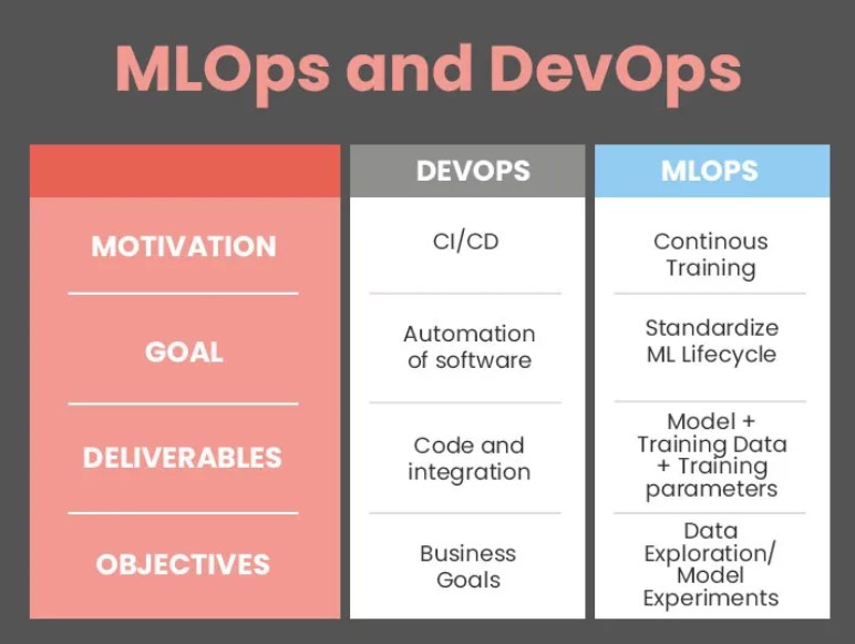
This is where a model registry stops being bookkeeping and becomes operational. A registry that versions every model alongside the metric baseline it was validated against — the reference distribution, the threshold set, the training data snapshot — is what lets a team roll back to a known-good version and recover from a regression within a single retraining cycle rather than a multi-week firefight. The whole loop is one stage of a larger system; where these pieces sit relative to CI/CD and data versioning is covered in our breakdown of the stages MLOps adds to a DevOps pipeline. Getting the metric baseline right before promotion is also why we treat pre-production serving benchmarks as part of the same discipline rather than a separate concern.
What thresholds and baselines fire a useful alert, not noise
Establishing the boundary between actionable signal and background variation poses the greatest operational challenge, far exceeding the difficulty of metric selection itself. A threshold that fires on every daily wobble trains your team to ignore alerts; a threshold set too loose never fires until it is a business incident. Both failure modes end in the same place: the metric is running and nobody trusts it.
A few principles hold up across the systems we have instrumented:
- Baseline against a distribution, not a point. Compare live metrics to the range observed during the model’s validated period, including its natural day-of-week and seasonal variance — not to a single golden number.
- Alert on sustained deviation, not single spikes. A one-hour drop can be a data-pipeline hiccup. A drop that persists across a rolling window is a model problem. Use windowed aggregation before you page anyone.
- Tier the severity. A soft threshold opens an investigation ticket; a hard threshold pages on-call or auto-triggers rollback. Collapsing these into one line is why alerting either screams or stays silent.
- Segment the metric. Aggregate accuracy can hold steady while the model quietly fails on a growing sub-population — a new region, a new device type, a new customer cohort. Per-segment monitoring catches the regression that the global average hides.
You can build all of this and still get burned if you never chose the right metric in the first place, which is why the sequence matters: metric selection, then baseline, then threshold, then alert. Doing it in that order is the difference between a monitoring system and an alerting theatre. These metrics are the sensing layer inside the wider discipline of MLOps as the operating model that keeps production machine learning healthy — a platform can only retrain, roll back, or page someone if a metric told it something moved. TechnoLynx works on exactly this kind of production hardening as part of our MLOps and applied AI engineering services, and the underlying stack choices are covered across our technologies work.
FAQ
What’s worth understanding about machine learning model performance metrics first?
Production monitoring demands metrics that surface drift, degradation, and business impact faster than batch evaluation ever could. You choose a metric that isolates the error your decision cares about, compute it on production traffic (or a computable proxy when labels are delayed), and wire it to a threshold that fires an alert. The number itself is only useful if something acts on it.
Which performance metrics matter for classification, regression, and ranking models, and how do you choose between them?
Classification with balanced classes can use accuracy; imbalanced classes need precision, recall, F1, or PR-AUC, and probability outputs need calibration metrics like log loss. Regression uses MAE or RMSE — RMSE when large errors are disproportionately costly. Ranking and recommendation use NDCG, MAP, or recall@k because position matters. The metric falls out of the output type and the decision the model feeds, not from a default.
How do offline validation metrics differ from the metrics you need to monitor in production?
Offline metrics are computed on a frozen, fully labelled test set — a clean-room snapshot. Production data shifts continuously and usually lacks immediate labels, so ground-truth metrics arrive delayed by label latency. That forces a two-tier strategy: fast label-free proxies like feature and prediction drift to catch changes early, and delayed ground-truth metrics to confirm actual regression.
How do performance metrics connect to drift detection and the trigger for automated retraining?
Drift is measured as a statistical distance between the training and live distributions (PSI, KS, Jensen–Shannon divergence). Crossing a threshold is the earliest computable evidence the model is out of its validated conditions, so it fires the investigation. A confirmed ground-truth regression then authorises retraining. Drift raises urgency; ground truth authorises action — retraining on every drift alert wastes compute.
What thresholds and baselines should you set so a metric fires a useful alert rather than noise?
Baseline against the metric’s observed range during the validated period, including natural seasonal variance, not a single number. Alert on sustained deviation across a rolling window rather than single spikes, tier severity so soft thresholds open tickets and hard ones page or roll back, and segment the metric so a failing sub-population is not hidden by the global average.
Why is a single headline metric like accuracy insufficient for production ML systems?
Accuracy collapses all error structure into one scalar and is misleading under class imbalance — a model predicting the majority class for a rare event can score near-perfect accuracy while catching nothing. It also cannot distinguish false positives from false negatives, which usually carry very different business costs. Production monitoring needs metrics that isolate the specific error a decision cares about.
A model with no production metric is not, in any credible sense, production-ready. That is precisely why metric coverage and drift-alerting maturity are scored inputs when we assess a system’s operational risk: the absence of a watched metric is not a gap in reporting — it is the failure class where accuracy loss becomes a business incident before anyone knew the model had moved.
Five metrics that expose production drift early
Early warning indicators—prediction entropy, feature null rates, and response-time percentiles—expose model degradation weeks ahead of any accuracy decline.