Run ollama run, watch a few tokens stream out, decide it feels fast, and mark the model production-ready. That is the benchmark most local LLM stacks get, and it is the reason so many of them quietly regress the moment something in the environment shifts. A driver update lands, a quantisation variant gets swapped in, a co-located batch job starts competing for the same GPU — and throughput halves without anyone noticing, because there was never a number to compare against.
An Ollama benchmark, done properly, is not a vibe check. It is a repeatable measurement harness: fixed prompt sets, concurrency sweeps, quantisation variants, run against the same hardware to produce tokens per second, time-to-first-token, and tail latency you can regression-test later. The output is a baseline, and the baseline is the thing your capacity and drift monitoring compares against. Without it, a local-serving stack becomes exactly the sort of load-bearing deployment that turns into a bottleneck nobody wired an alert for.
What does “benchmarking Ollama” actually mean in practice?
Two distinct meanings attach to “benchmark,” and failure to separate them undermines most naive measurement efforts. The first meaning is a one-off procurement check — does this model run acceptably on this box, yes or no. The second is an ongoing reference measurement you can rerun on demand and diff against history. Ollama, as a serving layer over llama.cpp and GGUF-quantised models, makes the first kind trivially easy and the second kind easy to skip.
In practice, a useful Ollama benchmark fixes everything you can fix and varies only the thing you are measuring. That means a frozen prompt set (so token counts are comparable), a defined generation length, a pinned model tag and quantisation level, and a warmed cache so you are not measuring cold-start model load as if it were inference latency. Once those are fixed, you sweep the variable of interest — concurrency, quantisation, or context length — and record the metrics at each point.
The distinction matters because the two meanings imply different artifacts. A procurement check produces a decision and then gets thrown away. A reference benchmark produces a stored baseline with a timestamp and an environment fingerprint, and that baseline is what makes a later regression visible. We treat the second kind as the default, because in our experience the stacks that survive contact with production are the ones that kept the number around.
Which metrics an Ollama benchmark should capture
Most operational insight concentrates in three metrics, each addressing separate performance dimensions. Tokens per second is the throughput number — how much text the model produces once it is going. Time-to-first-token is the responsiveness number — how long the user stares at a blank screen before anything appears. Tail latency (p95 and p99) is the fairness number — what the unlucky requests experience while the median request looks fine.
These diverge sharply under load, which is the whole reason to measure them separately. A single-request benchmark on a warm GPU might show time-to-first-token in the tens to low hundreds of milliseconds and a healthy tokens-per-second figure, and you might conclude the model is fast. Push concurrency up and the picture inverts: throughput per request drops as the GPU time-slices between streams, time-to-first-token climbs because requests queue behind each other, and the p99 detaches from the median entirely. The median can look unchanged while the tail doubles.
| Metric | Question it answers | What degrades it under load |
|---|---|---|
| Tokens/sec (per request) | How fast does text stream once generation starts? | Concurrency splitting GPU compute; smaller effective batch per stream |
| Tokens/sec (aggregate) | How much total work does the box do? | VRAM exhaustion forcing shorter context or eviction |
| Time-to-first-token | How responsive does it feel? | Request queuing; prompt-processing (prefill) contention |
| p95 / p99 latency | What do unlucky requests experience? | Head-of-line blocking; co-located workload contention |
The aggregate-versus-per-request split is the one teams most often miss. A box can serve more total tokens per second as you add concurrency while every individual user gets slower — because you have traded per-request latency for throughput. Whether that trade is acceptable is a product decision, not a benchmark result, but you cannot make the decision without both numbers on the table. This is the same principle behind treating production performance metrics as things you track continuously rather than measure once: the point-in-time reading is nearly meaningless without the distribution and the trend around it.
How quantisation and VRAM constraints move the numbers
Quantisation exerts more influence over Ollama benchmark outcomes than any other factor, simultaneously shifting multiple dimensions in ways that obscure true cause and effect. A model served at Q4_K_M uses roughly half the VRAM of the same model at Q8, which changes not just memory headroom but how much of the model and KV cache stay resident on the GPU rather than spilling. When part of the model offloads to system RAM, tokens-per-second can collapse by an order of magnitude, and the benchmark will read that as “the model is slow” when the real cause is a memory-fit problem.
The relationship is not linear and it is not the same across hardware. On a GPU with ample VRAM for the model, dropping from Q8 to Q4 may buy modest throughput and negligible quality loss; on a VRAM-constrained box it may be the difference between fully-resident inference and painful CPU offload — a throughput swing far larger than the quantisation arithmetic alone suggests (observed across serving configurations we have profiled; not a published benchmark). That is why the quantisation sweep and the VRAM budget have to be measured together, on the target hardware, rather than reasoned about in the abstract.
None of these numbers mean anything divorced from the silicon underneath them. A tokens-per-second figure is a statement about a model and a GPU and a driver stack, which is why readers sizing compute for local serving should read them against the GPU infrastructure that training and serving workloads actually run on. The same Q4 model on two different accelerators is two different benchmarks. Our own technologies practice treats the executor — hardware plus software stack — as the real unit of measurement, not the model tag alone.
How do you run a repeatable Ollama benchmark instead of a one-off eyeball test?
Control every variable outside your measurement target to achieve consistent results. The eyeball test fails not because a human is bad at noticing slowness but because the human is comparing against a memory, not a recorded baseline, and comparing across an environment that has silently changed. A repeatable harness fixes that with a short discipline checklist.
- Freeze the prompt set. Use a fixed corpus of prompts with known, stable token counts so that tokens-per-second is comparable run to run. Random or user-supplied prompts make every run a different experiment.
- Warm before you measure. The first request after
ollama runincludes model load and cache population. Discard warm-up requests; measure steady state. - Pin the model and quantisation tag explicitly.
llama3:8bis not a version. Record the exact tag, digest, and quantisation so a later run is comparing like with like. - Sweep concurrency deliberately. Measure at 1, then at your expected steady-state concurrency, then above it. The curve — not any single point — is the result.
- Fingerprint the environment. Record GPU model, driver version, Ollama version, and whether any other workload shared the device. A regression you cannot attribute to a changed variable is not actionable.
- Store the result with a timestamp. The baseline only has value if it persists. A benchmark you ran and forgot is a procurement check, not a reference.
The concurrency sweep deserves emphasis because it is where the one-off test is most misleading. Single-stream numbers flatter every configuration. It is only when you plot latency and throughput against concurrent load that the knee in the curve appears — the point where adding one more concurrent user degrades everyone’s experience faster than it adds aggregate throughput. That knee is your real capacity ceiling, and it is invisible to any benchmark that runs one request at a time.
Feeding the baseline into drift and capacity monitoring
Ephemeral benchmarks executed in disposable terminal sessions deliver incomplete value. The value compounds when the baseline becomes the reference that continuous monitoring compares against. This is where an Ollama benchmark stops being a serving concern and becomes an MLOps concern — the operational layer that turns a model that works into a service that keeps working.
The mechanism is straightforward once the baseline exists. You record the benchmark’s tokens-per-second and p95 latency as the expected operating envelope, then instrument the live serving path to emit the same metrics. When production tokens-per-second drops below the baseline by more than a defined threshold, that is an alert — and crucially, it is an alert you can trust, because you know what “normal” looked like on this exact hardware and software combination. Without the baseline, a 40% throughput regression from a driver update looks like ordinary variance; with it, the regression is a numbered deviation from a known reference.
This is the same discipline that governs what to track for model performance in production: the monitoring is only as good as the baseline it compares against. A drift detector with no reference distribution cannot tell you the distribution drifted. A capacity monitor with no benchmarked ceiling cannot tell you you are approaching it. The benchmark is not a one-time artifact you file and forget — it is the calibration for everything that watches the system afterward.
Turning benchmark numbers into a capacity model
Translating raw measurements into cost projections represents the last critical step. A concurrency sweep gives you a curve of latency and throughput against concurrent users; the point where p95 latency crosses your product’s acceptable threshold is your per-box concurrent-user ceiling. Divide expected peak concurrent users by that ceiling and you have how many boxes you need — a number derived from measurement rather than from over-provisioning by 2–3× “to be safe.”
Consider a worked example with explicit assumptions. Suppose a benchmark shows a given GPU sustains acceptable p95 latency up to eight concurrent generation streams, and aggregate throughput at that point is on the order of a few hundred tokens per second. If your product’s peak is forty concurrent users, you need roughly five such boxes to hold latency, and your cost per thousand tokens is the hourly cost of those boxes divided by their aggregate token output (illustrative arithmetic; substitute your measured numbers). Change the quantisation and the ceiling moves; change the GPU and the whole curve moves. The capacity model is only as honest as the benchmark feeding it.
That cost-per-thousand-tokens figure is the number that survives into a budget conversation, and it is the number a procurement or readiness review actually wants. A benchmarked, regression-tested local-serving stack is a documented strength in an MLOps-maturity assessment; an unmeasured one is a documented risk variable — a load-bearing deployment with no known baseline. Which of the two you have is decided before the model goes live, not after the first incident — the same framing MLOps: The Operating Model That Keeps Production Machine Learning Healthy applies to a full production system, just scoped down to one serving stack’s throughput number.
FAQ
What does working with ollama-benchmark involve in practice?
Running fixed prompts against a pinned model and quantization, Ollama benchmarks capture tokens per second, time-to-first-token, and tail latency on specified hardware. In practice it means treating measurement as a repeatable harness rather than a single ollama run you eyeball — the output is a stored baseline with an environment fingerprint that later runs can be compared against.
What metrics should an Ollama benchmark capture — tokens/sec, time-to-first-token, p95/p99 latency, and how do they differ under load?
Capture per-request tokens/sec (streaming speed), aggregate tokens/sec (total box throughput), time-to-first-token (responsiveness), and p95/p99 latency (tail behaviour). Under load these diverge: aggregate throughput can rise while per-request speed falls, time-to-first-token climbs as requests queue, and the p99 detaches from the median. A single-request reading hides all of this.
How do model quantisation level and GPU/VRAM constraints change Ollama benchmark results?
Quantisation is the biggest single lever — a lower-precision variant uses less VRAM, which changes how much of the model and KV cache stay resident on the GPU. When memory doesn’t fit and layers offload to system RAM, throughput can collapse far beyond what the precision change alone implies, so quantisation and VRAM budget must be measured together on the target hardware.
How do you run a repeatable Ollama benchmark with fixed prompt sets and concurrency sweeps rather than a one-off eyeball test?
Freeze the prompt set so token counts are comparable, discard warm-up requests to measure steady state, pin the exact model tag and quantisation, sweep concurrency from one request up past expected load, and fingerprint the environment (GPU, driver, Ollama version). Store each result with a timestamp — the curve across concurrency, not any single point, is the actual result.
How does a serving benchmark baseline feed into MLOps drift and capacity monitoring so throughput regressions trigger an alert?
The benchmark’s tokens/sec and p95 latency become the expected operating envelope; you instrument the live serving path to emit the same metrics and alert when production drops below the baseline by a set threshold. Because you know what normal looked like on this exact hardware and software, a driver-induced regression reads as a numbered deviation rather than ordinary variance.
How do you translate Ollama benchmark numbers into a capacity model — concurrent users, hardware cost per thousand tokens?
The concurrency sweep gives the point where p95 latency crosses your acceptable threshold — that is your per-box concurrent-user ceiling. Divide expected peak concurrency by that ceiling for box count, then divide those boxes’ hourly cost by their aggregate token output for cost per thousand tokens. The model is only as honest as the benchmark feeding it, and it moves with quantisation and GPU choice.
The open question for most teams is not whether their local LLM stack is fast today — it is whether they would know if it stopped being fast tomorrow. A benchmark you can rerun and diff is the difference between catching a throughput regression in a controlled run and catching it in a production incident, and it is a concrete input to how our services scope MLOps readiness rather than a checkbox you tick once and forget.
Benchmarking Ollama with representative prompt distributions
Uniform 512-token synthetic prompts will inflate throughput estimates by 30–40% (as a sizing estimate) relative to production workloads mixing long-context retrieval and variable-length multi-turn dialogue. The teams that do tend to ship the boring, correct version first.